This page was generated from docs/notebooks/02_energy_analysis.ipynb.
Energy Analysis
Energy Analysis
Energy landscapes provide a quantitative measure of cellular state stability in the Hopfield network framework.
Energy Function
The total energy is decomposed into three components:
Where:
Computing Energies
Visualization
scHopfield provides comprehensive plotting functions for all analysis results.
Energy Plots
See energy_analysis for details.
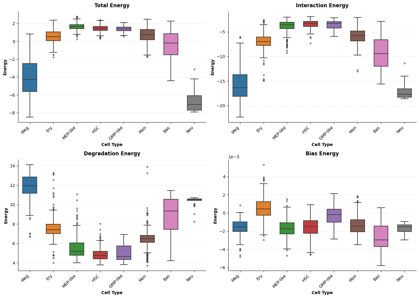
The scHopfield energy functional decomposes into three biologically interpretable
components:
E_interaction: Energy stored in gene–gene regulatory interactions
E_degradation: Energy stored in mRNA decay terms
E_bias: Energy stored in external input / basal expression bias
Lower total energy ≈ more stable attractor state. This notebook shows how to
compute, visualise, and interpret these energies.
Setup
[1]:
import itertools

import matplotlib.pyplot as plt
import numpy as np
import pandas as pd
import scanpy as sc
import scHopfield as sch

import warnings
warnings.filterwarnings('ignore', category=FutureWarning)

# Assumes the model was saved in notebook 01
DATA_PATH  = './scratch/Data/'
DATASET_FILE = 'hematopoiesis.h5ad'
MODEL_FILE = 'model.h5sch'

CLUSTER_KEY = 'cell_type'
SPLICED_KEY  = 'M_t'

CELL_TYPE_ORDER = ['Meg', 'Ery', 'MEP-like', 'HSC', 'GMP-like', 'Mon', 'Bas', 'Neu']

adata = sc.read_h5ad(DATA_PATH + DATASET_FILE)
adata = sch.tl.load_model(adata, MODEL_FILE)
print(adata)


# Set seed for reproducibility
np.random.seed(42)
/home/bernaljp/miniconda3/envs/SCH/lib/python3.11/site-packages/louvain/__init__.py:54: UserWarning: pkg_resources is deprecated as an API. See https://setuptools.pypa.io/en/latest/pkg_resources.html. The pkg_resources package is slated for removal as early as 2025-11-30. Refrain from using this package or pin to Setuptools<81.
  from pkg_resources import get_distribution, DistributionNotFound
/tmp/ipykernel_1221845/3037205977.py:23: UserWarning: adata has 1956 genes but the model was trained on 1728.  A subsetted copy is being returned; the original adata is NOT modified.  Reassign the return value:
    adata = sch.tl.load_model(adata, filename)
  adata = sch.tl.load_model(adata, MODEL_FILE)
Model loaded from 'model.h5sch'  |  clusters=['Bas', 'Ery', 'GMP-like', 'HSC', 'MEP-like', 'Meg', 'Mon', 'Neu', 'all']  |  genes=1728
AnnData object with n_obs × n_vars = 1947 × 1728
    obs: 'batch', 'time', 'cell_type', 'nGenes', 'nCounts', 'pMito', 'pass_basic_filter', 'new_Size_Factor', 'initial_new_cell_size', 'total_Size_Factor', 'initial_total_cell_size', 'spliced_Size_Factor', 'initial_spliced_cell_size', 'unspliced_Size_Factor', 'initial_unspliced_cell_size', 'Size_Factor', 'initial_cell_size', 'ntr', 'cell_cycle_phase', 'leiden', 'control_point_pca', 'inlier_prob_pca', 'obs_vf_angle_pca', 'pca_ddhodge_div', 'pca_ddhodge_potential', 'acceleration_pca', 'curvature_pca', 'n_counts', 'mt_frac', 'jacobian_det_pca', 'manual_selection', 'divergence_pca', 'curv_leiden', 'curv_louvain', 'SPI1->GATA1_jacobian', 'jacobian', 'umap_ori_leiden', 'umap_ori_louvain', 'umap_ddhodge_div', 'umap_ddhodge_potential', 'curl_umap', 'divergence_umap', 'acceleration_umap', 'control_point_umap_ori', 'inlier_prob_umap_ori', 'obs_vf_angle_umap_ori', 'curvature_umap_ori'
    var: 'gene_name', 'gene_id', 'nCells', 'nCounts', 'pass_basic_filter', 'use_for_pca', 'frac', 'ntr', 'time_3_alpha', 'time_3_beta', 'time_3_gamma', 'time_3_half_life', 'time_3_alpha_b', 'time_3_alpha_r2', 'time_3_gamma_b', 'time_3_gamma_r2', 'time_3_gamma_logLL', 'time_3_delta_b', 'time_3_delta_r2', 'time_3_bs', 'time_3_bf', 'time_3_uu0', 'time_3_ul0', 'time_3_su0', 'time_3_sl0', 'time_3_U0', 'time_3_S0', 'time_3_total0', 'time_3_beta_k', 'time_3_gamma_k', 'time_5_alpha', 'time_5_beta', 'time_5_gamma', 'time_5_half_life', 'time_5_alpha_b', 'time_5_alpha_r2', 'time_5_gamma_b', 'time_5_gamma_r2', 'time_5_gamma_logLL', 'time_5_bs', 'time_5_bf', 'time_5_uu0', 'time_5_ul0', 'time_5_su0', 'time_5_sl0', 'time_5_U0', 'time_5_S0', 'time_5_total0', 'time_5_beta_k', 'time_5_gamma_k', 'use_for_dynamics', 'gamma', 'gamma_r2', 'use_for_transition', 'gamma_k', 'gamma_b', 'I_Bas', 'I_Ery', 'I_GMP-like', 'I_HSC', 'I_MEP-like', 'I_Meg', 'I_Mon', 'I_Neu', 'I_all', 'scHopfield_used', 'sigmoid_exponent', 'sigmoid_mse', 'sigmoid_offset', 'sigmoid_threshold'
    uns: 'PCs', 'VecFld_pca', 'VecFld_umap', 'X_umap_neighbors', 'cell_phase_genes', 'cell_type_colors', 'dynamics', 'explained_variance_ratio_', 'feature_selection', 'grid_velocity_pca', 'grid_velocity_umap', 'grid_velocity_umap_ori_perturbation', 'grid_velocity_umap_test', 'jacobian_pca', 'leiden', 'neighbors', 'pca_mean', 'pp', 'response', 'scHopfield'
    obsm: 'X', 'X_pca', 'X_pca_SparseVFC', 'X_umap', 'X_umap_SparseVFC', 'X_umap_ori_perturbation', 'X_umap_test', 'acceleration_pca', 'acceleration_umap', 'cell_cycle_scores', 'curvature_pca', 'curvature_umap', 'j_delta_x_perturbation', 'velocity_pca', 'velocity_pca_SparseVFC', 'velocity_umap', 'velocity_umap_SparseVFC', 'velocity_umap_ori_perturbation', 'velocity_umap_test'
    layers: 'M_n', 'M_nn', 'M_t', 'M_tn', 'M_tt', 'X_new', 'X_total', 'velocity_alpha_minus_gamma_s'
    obsp: 'X_umap_connectivities', 'X_umap_distances', 'connectivities', 'cosine_transition_matrix', 'distances', 'fp_transition_rate', 'moments_con', 'pca_ddhodge', 'perturbation_transition_matrix', 'umap_ddhodge'
    varp: 'W_Bas', 'W_Ery', 'W_GMP-like', 'W_HSC', 'W_MEP-like', 'W_Meg', 'W_Mon', 'W_Neu', 'W_all'
2.1 Compute & Decompose Energies
[2]:
sch.tl.compute_energies(adata, cluster_key=CLUSTER_KEY, spliced_key=SPLICED_KEY)

# Inspect stored energy columns
energy_cols = ['energy_total', 'energy_interaction', 'energy_degradation', 'energy_bias']
print(adata.obs[energy_cols].describe())
       energy_total  energy_interaction  energy_degradation  energy_bias
count   1947.000000         1947.000000         1947.000000  1947.000000
mean       0.465193           -6.238026            6.703232    -0.000013
std        2.017105            4.142948            2.293970     0.000014
min       -8.506401          -22.371951            3.737046    -0.000058
25%        0.257570           -7.225530            4.937362    -0.000021
50%        1.199007           -4.855515            6.226903    -0.000014
75%        1.606413           -3.356720            7.367836    -0.000005
max        2.778031           -1.868195           14.112776     0.000053
[3]:
# Summary statistics per cell type (including coefficient of variation)
summary = adata.obs[[CLUSTER_KEY] + energy_cols].groupby(CLUSTER_KEY).describe()
for energy in energy_cols:
    summary[(energy, 'cv')] = summary[(energy, 'std')] / summary[(energy, 'mean')]

print("\nTotal energy statistics:")
print(summary['energy_total'].round(3))
Total energy statistics:
           count   mean    std    min    25%    50%    75%    max     cv
cell_type
Bas        177.0 -0.475  1.625 -4.416 -1.506 -0.197  0.840  2.274 -3.419
Ery        234.0  0.538  0.726 -1.788  0.057  0.502  1.054  2.369  1.349
GMP-like   161.0  1.386  0.306  0.547  1.190  1.391  1.593  2.092  0.221
HSC        309.0  1.433  0.374  0.309  1.227  1.465  1.663  2.383  0.261
MEP-like   457.0  1.659  0.350  0.224  1.430  1.656  1.871  2.778  0.211
Meg        154.0 -4.099  2.206 -8.506 -5.636 -4.294 -2.506  0.812 -0.538
Mon        423.0  0.672  0.888 -1.749  0.173  0.757  1.325  2.478  1.322
Neu         32.0 -6.661  1.309 -7.924 -7.730 -7.065 -6.085 -3.137 -0.196
2.2 Energy Boxplots by Cell Type
[4]:
adata
[4]:
AnnData object with n_obs × n_vars = 1947 × 1728
    obs: 'batch', 'time', 'cell_type', 'nGenes', 'nCounts', 'pMito', 'pass_basic_filter', 'new_Size_Factor', 'initial_new_cell_size', 'total_Size_Factor', 'initial_total_cell_size', 'spliced_Size_Factor', 'initial_spliced_cell_size', 'unspliced_Size_Factor', 'initial_unspliced_cell_size', 'Size_Factor', 'initial_cell_size', 'ntr', 'cell_cycle_phase', 'leiden', 'control_point_pca', 'inlier_prob_pca', 'obs_vf_angle_pca', 'pca_ddhodge_div', 'pca_ddhodge_potential', 'acceleration_pca', 'curvature_pca', 'n_counts', 'mt_frac', 'jacobian_det_pca', 'manual_selection', 'divergence_pca', 'curv_leiden', 'curv_louvain', 'SPI1->GATA1_jacobian', 'jacobian', 'umap_ori_leiden', 'umap_ori_louvain', 'umap_ddhodge_div', 'umap_ddhodge_potential', 'curl_umap', 'divergence_umap', 'acceleration_umap', 'control_point_umap_ori', 'inlier_prob_umap_ori', 'obs_vf_angle_umap_ori', 'curvature_umap_ori', 'energy_total', 'energy_interaction', 'energy_degradation', 'energy_bias'
    var: 'gene_name', 'gene_id', 'nCells', 'nCounts', 'pass_basic_filter', 'use_for_pca', 'frac', 'ntr', 'time_3_alpha', 'time_3_beta', 'time_3_gamma', 'time_3_half_life', 'time_3_alpha_b', 'time_3_alpha_r2', 'time_3_gamma_b', 'time_3_gamma_r2', 'time_3_gamma_logLL', 'time_3_delta_b', 'time_3_delta_r2', 'time_3_bs', 'time_3_bf', 'time_3_uu0', 'time_3_ul0', 'time_3_su0', 'time_3_sl0', 'time_3_U0', 'time_3_S0', 'time_3_total0', 'time_3_beta_k', 'time_3_gamma_k', 'time_5_alpha', 'time_5_beta', 'time_5_gamma', 'time_5_half_life', 'time_5_alpha_b', 'time_5_alpha_r2', 'time_5_gamma_b', 'time_5_gamma_r2', 'time_5_gamma_logLL', 'time_5_bs', 'time_5_bf', 'time_5_uu0', 'time_5_ul0', 'time_5_su0', 'time_5_sl0', 'time_5_U0', 'time_5_S0', 'time_5_total0', 'time_5_beta_k', 'time_5_gamma_k', 'use_for_dynamics', 'gamma', 'gamma_r2', 'use_for_transition', 'gamma_k', 'gamma_b', 'I_Bas', 'I_Ery', 'I_GMP-like', 'I_HSC', 'I_MEP-like', 'I_Meg', 'I_Mon', 'I_Neu', 'I_all', 'scHopfield_used', 'sigmoid_exponent', 'sigmoid_mse', 'sigmoid_offset', 'sigmoid_threshold'
    uns: 'PCs', 'VecFld_pca', 'VecFld_umap', 'X_umap_neighbors', 'cell_phase_genes', 'cell_type_colors', 'dynamics', 'explained_variance_ratio_', 'feature_selection', 'grid_velocity_pca', 'grid_velocity_umap', 'grid_velocity_umap_ori_perturbation', 'grid_velocity_umap_test', 'jacobian_pca', 'leiden', 'neighbors', 'pca_mean', 'pp', 'response', 'scHopfield'
    obsm: 'X', 'X_pca', 'X_pca_SparseVFC', 'X_umap', 'X_umap_SparseVFC', 'X_umap_ori_perturbation', 'X_umap_test', 'acceleration_pca', 'acceleration_umap', 'cell_cycle_scores', 'curvature_pca', 'curvature_umap', 'j_delta_x_perturbation', 'velocity_pca', 'velocity_pca_SparseVFC', 'velocity_umap', 'velocity_umap_SparseVFC', 'velocity_umap_ori_perturbation', 'velocity_umap_test'
    layers: 'M_n', 'M_nn', 'M_t', 'M_tn', 'M_tt', 'X_new', 'X_total', 'velocity_alpha_minus_gamma_s', 'sigmoid'
    obsp: 'X_umap_connectivities', 'X_umap_distances', 'connectivities', 'cosine_transition_matrix', 'distances', 'fp_transition_rate', 'moments_con', 'pca_ddhodge', 'perturbation_transition_matrix', 'umap_ddhodge'
    varp: 'W_Bas', 'W_Ery', 'W_GMP-like', 'W_HSC', 'W_MEP-like', 'W_Meg', 'W_Mon', 'W_Neu', 'W_all'
[5]:
# Retrieve cell-type colours from the dataset (or define your own dict)
# colors = {ct: f'C{i}' for i, ct in enumerate(CELL_TYPE_ORDER)}
colors = dict(zip(CELL_TYPE_ORDER, adata.uns['cell_type_colors']))

# All four energy components
sch.pl.plot_energy_boxplots(
    adata,
    cluster_key=CLUSTER_KEY,
    order=CELL_TYPE_ORDER,
    colors=colors
)
plt.show()
/home/bernaljp/packages/scHopfield/scHopfield/plotting/energy.py:204: UserWarning: FixedFormatter should only be used together with FixedLocator
  ax.set_xticklabels(ax.get_xticklabels(), rotation=45, ha='right')
/home/bernaljp/packages/scHopfield/scHopfield/plotting/energy.py:204: UserWarning: FixedFormatter should only be used together with FixedLocator
  ax.set_xticklabels(ax.get_xticklabels(), rotation=45, ha='right')
/home/bernaljp/packages/scHopfield/scHopfield/plotting/energy.py:204: UserWarning: FixedFormatter should only be used together with FixedLocator
  ax.set_xticklabels(ax.get_xticklabels(), rotation=45, ha='right')
/home/bernaljp/packages/scHopfield/scHopfield/plotting/energy.py:204: UserWarning: FixedFormatter should only be used together with FixedLocator
  ax.set_xticklabels(ax.get_xticklabels(), rotation=45, ha='right')
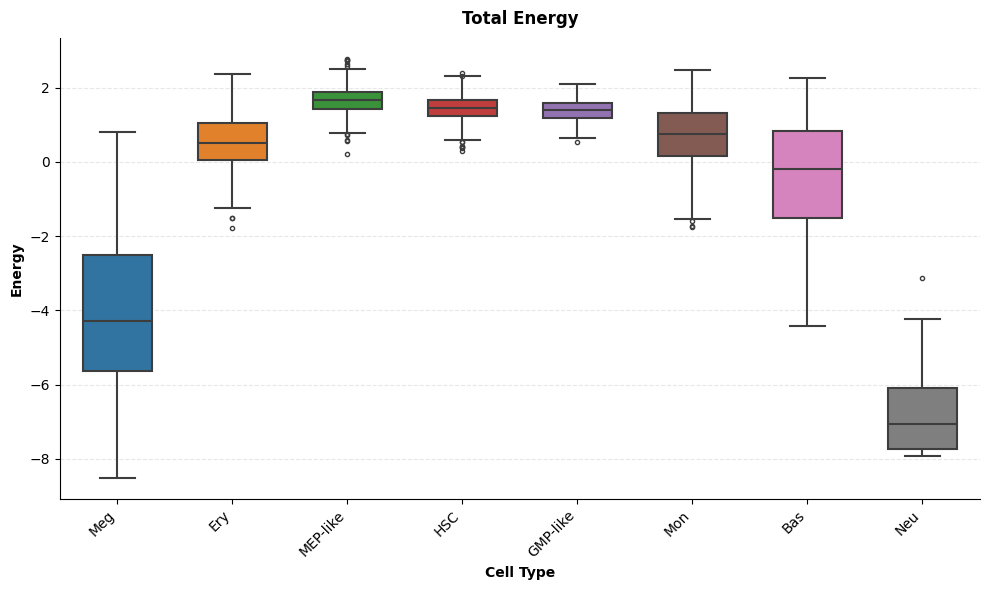
[6]:
# Total energy only
sch.pl.plot_energy_boxplots(
    adata,
    cluster_key=CLUSTER_KEY,
    plot_energy='total',
    order=CELL_TYPE_ORDER,
    colors=[colors[k] for k in CELL_TYPE_ORDER]
)
plt.show()
/home/bernaljp/packages/scHopfield/scHopfield/plotting/energy.py:204: UserWarning: FixedFormatter should only be used together with FixedLocator
  ax.set_xticklabels(ax.get_xticklabels(), rotation=45, ha='right')
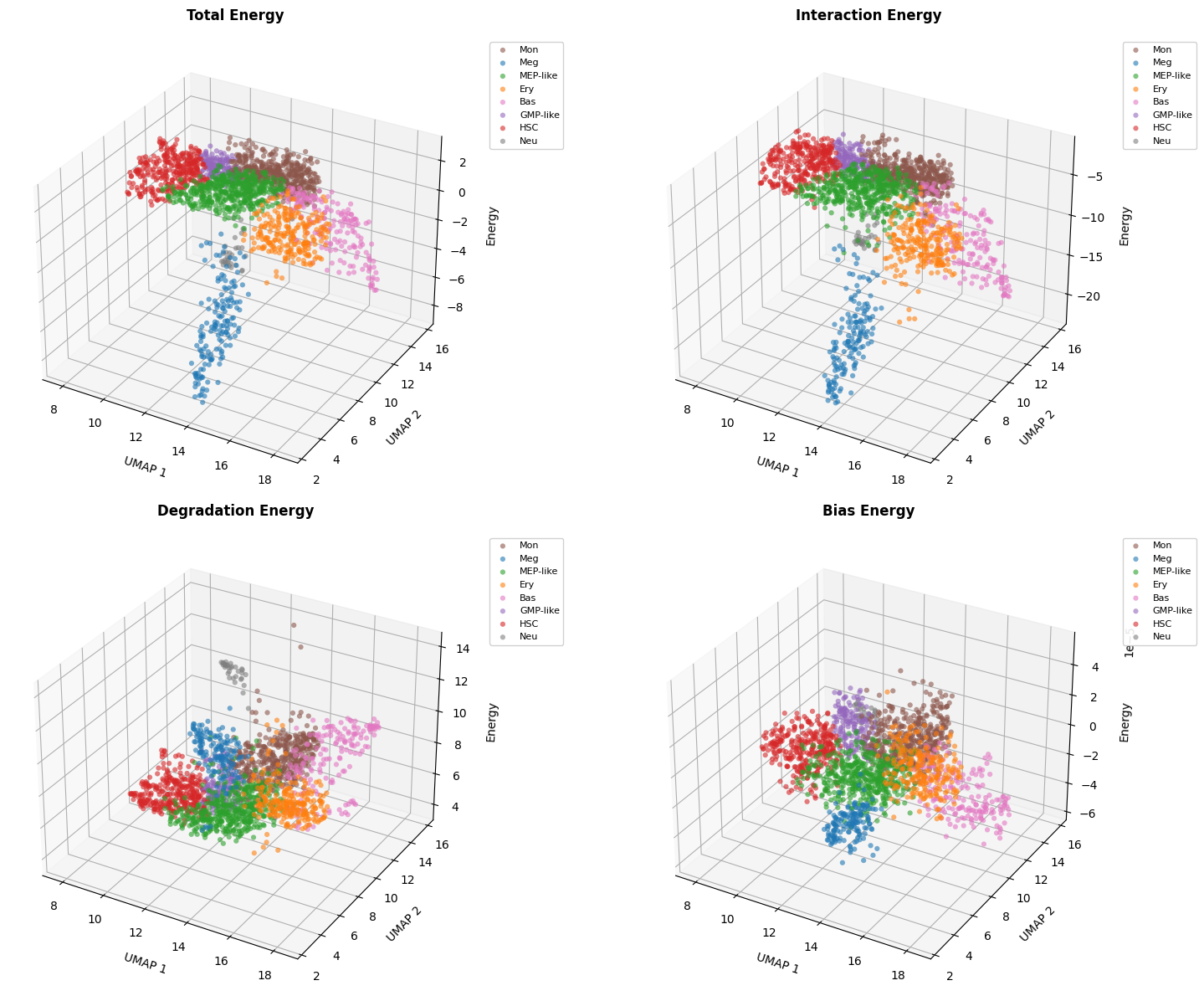
2.3 Energy on UMAP
[7]:
# Scatter plots of each energy component overlaid on UMAP embedding
sch.pl.plot_energy_scatters(
    adata,
    cluster_key=CLUSTER_KEY,
    basis='umap',
    show_legend=True,
    colors=colors,
)
plt.show()
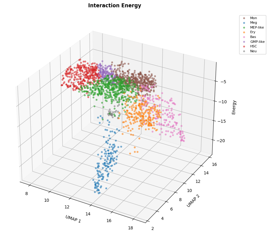
[8]:
# Interaction energy only
sch.pl.plot_energy_scatters(
    adata,
    cluster_key=CLUSTER_KEY,
    plot_energy='interaction',
    colors=colors,
)
plt.show()
2.4 Energy–Gene Correlations
Identifies which genes drive energy differences across cell types.
[9]:
sch.tl.energy_gene_correlation(
    adata,
    spliced_key=SPLICED_KEY,
    cluster_key=CLUSTER_KEY
)

# Tabulate top correlated genes
df_correlations = sch.tl.get_correlation_table(
    adata,
    cluster_key=CLUSTER_KEY,
    energy_type='total',
    n_top_genes=100,
    order=CELL_TYPE_ORDER
)
df_correlations.head(10)
/home/bernaljp/miniconda3/envs/SCH/lib/python3.11/site-packages/numpy/lib/function_base.py:2897: RuntimeWarning: invalid value encountered in divide
  c /= stddev[:, None]
/home/bernaljp/miniconda3/envs/SCH/lib/python3.11/site-packages/numpy/lib/function_base.py:2898: RuntimeWarning: invalid value encountered in divide
  c /= stddev[None, :]
[9]:
| Meg | Ery | MEP-like | HSC | GMP-like | Mon | Bas | Neu | |||||||||
|---|---|---|---|---|---|---|---|---|---|---|---|---|---|---|---|---|
| Gene | Correlation | Gene | Correlation | Gene | Correlation | Gene | Correlation | Gene | Correlation | Gene | Correlation | Gene | Correlation | Gene | Correlation | |
| 0 | FBL | 0.807304 | FABP5 | 0.665676 | PRSS57 | 0.315137 | CCDC137 | 0.482047 | CITED2 | 0.434898 | ELF1 | 0.649138 | EXO1 | 0.807626 | FBL | 0.900663 |
| 1 | PHB2 | 0.778194 | CD33 | 0.650139 | IL17RB | 0.307605 | NOP9 | 0.436700 | ITGA2B | 0.412077 | HERC2P9 | 0.563224 | FABP5 | 0.742007 | ERG | 0.882317 |
| 2 | ZNRF1 | 0.775508 | RASSF2 | 0.641904 | CHD3 | 0.284941 | FUCA2 | 0.425116 | FCER1A | 0.400928 | TOP2A | 0.536342 | PHB2 | 0.725082 | ACSS1 | 0.868937 |
| 3 | RPL18A | 0.748102 | PALM2AKAP2 | 0.618501 | RAB20 | 0.280315 | SOD2 | 0.425081 | HDC | 0.399843 | KANTR | 0.532998 | RPL18A | 0.711273 | GFI1 | 0.866927 |
| 4 | HMGB3 | 0.744607 | IL2RG | 0.611712 | PEX6 | 0.279536 | PTCD1 | 0.420303 | AL157895.1 | 0.384206 | STAT3 | 0.531445 | ARV1 | 0.693583 | KLHDC2 | 0.861760 |
| 5 | RPL35 | 0.731323 | SATB1 | 0.597738 | RASSF2 | 0.272160 | COTL1 | 0.393799 | CPA3 | 0.371276 | ASPM | 0.526317 | MFSD2B | 0.679917 | POLR1C | 0.840239 |
| 6 | RPUSD4 | 0.723665 | MBOAT7 | 0.560575 | SRGN | 0.269023 | PSEN1 | 0.387846 | DDIT4 | 0.370603 | HERC2P3 | 0.515384 | DDX41 | 0.675017 | AQP3 | 0.826446 |
| 7 | RECQL4 | 0.713247 | DBN1 | 0.556944 | USE1 | 0.268064 | RECQL4 | 0.387596 | GATA2 | 0.369129 | CD34 | 0.507963 | FBL | 0.672615 | ASPM | 0.824554 |
| 8 | EIF3K | 0.710026 | AC244502.1 | 0.550963 | CEBPA | 0.266089 | MFSD2B | 0.384711 | HPGDS | 0.366681 | CASP7 | 0.504359 | GPI | 0.672221 | ERCC6 | 0.823418 |
| 9 | HPGDS | 0.703534 | LPCAT2 | 0.549897 | CEACAM1 | 0.259691 | DDX41 | 0.379453 | ZFPM1 | 0.366653 | RDX | 0.500153 | APRT | 0.667679 | INKA1 | 0.822812 |
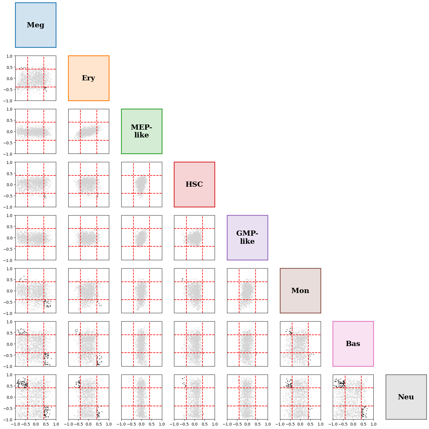
[10]:
# Pairwise scatter plots (all combinations of cell-type pairs)
sch.pl.plot_correlations_grid(
    adata,
    cluster_key=CLUSTER_KEY,
    energy='total',
    order=CELL_TYPE_ORDER,
    colors=colors,
    x_low=-0.4, x_high=0.4,
    y_low=-0.4, y_high=0.4
)
plt.show()
[11]:
# Highlight specific cell-type pairs
fig, ax = plt.subplots(1, 3, figsize=(18, 6), tight_layout=True)

sch.pl.plot_gene_correlation_scatter(
    adata, 'Meg', 'Ery',
    cluster_key=CLUSTER_KEY, energy='total',
    annotate=6, ax=ax[0],
    clus1_low=-0.4, clus1_high=0.4,
    clus2_low=-0.4, clus2_high=0.4
)
sch.pl.plot_gene_correlation_scatter(
    adata, 'Neu', 'Bas',
    cluster_key=CLUSTER_KEY, energy='total',
    annotate=6, ax=ax[1]
)
sch.pl.plot_gene_correlation_scatter(
    adata, 'Neu', 'Mon',
    cluster_key=CLUSTER_KEY, energy='total',
    annotate=6, ax=ax[2]
)
plt.show()
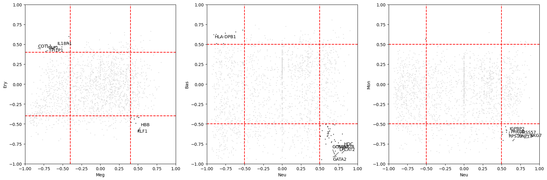
2.5 Corner Gene Identification
“Corner genes” have high-magnitude correlation with one cell type and opposing
(or low) correlation with another — these are candidate lineage-specific
regulatory genes.
[12]:
import itertools
genes_mask  = sch._utils.io.get_genes_used(adata)
gene_names  = adata.var.index[genes_mask]

# Build per-cluster correlation arrays
correlation = {}
for cluster in CELL_TYPE_ORDER:
    col = f'correlation_total_{cluster}'
    if col in adata.var.columns:
        correlation[cluster] = adata.var[col].values[genes_mask]

# Thresholds for "corner" classification
clus1_low  = -0.4
clus1_high =  0.4
clus2_low  = -0.4
clus2_high =  0.4
nn = 5   # top-n genes per pair

corner_genes = np.array([])

for corr1, corr2 in itertools.combinations(CELL_TYPE_ORDER, 2):
    if corr1 not in correlation or corr2 not in correlation:
        continue

    c1 = correlation[corr1]
    c2 = correlation[corr2]

    mask_corner = np.logical_or(
        np.logical_and(c1 >= clus1_high, c2 <= clus2_low),
        np.logical_and(c1 <= clus1_low,  c2 >= clus2_high)
    )

    idxs = np.where(mask_corner)[0]
    top  = np.argsort(c1[idxs] ** 2 + c2[idxs] ** 2)[-nn:]
    corner_genes = np.concatenate((corner_genes, gene_names[idxs[top]]))

corner_genes = np.unique(corner_genes)
print(f"Found {len(corner_genes)} corner genes:")
print(corner_genes)
Found 54 corner genes:
['ACSS1' 'AHNAK' 'ARL6IP5' 'ASPM' 'AURKA' 'AURKAIP1' 'CENPE' 'CITED2'
 'CNPY3' 'CORO1A' 'COTL1' 'CPA3' 'CYBA' 'E2F4' 'EIF3K' 'FUCA2' 'GATA2'
 'GCSAML' 'GFI1' 'HDC' 'HEMGN' 'HERC5' 'HLA-DMA' 'HLA-DPB1' 'HLA-DQB1'
 'HLA-DRB6' 'HPGDS' 'IL18R1' 'IL2RG' 'ITGA2B' 'KLF1' 'LMO2' 'LPCAT2'
 'LTBP1' 'NKG7' 'PF4' 'PRICKLE1' 'RAB27B' 'RABGGTA' 'RASSF2' 'RPL35'
 'RPS19' 'RPS21' 'SEMA7A' 'SLC1A4' 'SNCA' 'SOD2' 'STON2' 'SUN2' 'TAP1'
 'TMEM273' 'TOP2A' 'TPI1P1' 'ZNF263']
[13]:
# Visualise corner gene correlation table
df_corr_corners = pd.DataFrame.from_dict(correlation, orient='columns')
df_corr_corners.index = gene_names
df_corr_corners = df_corr_corners.loc[corner_genes]
df_corr_corners.round(3)
[13]:
| Meg | Ery | MEP-like | HSC | GMP-like | Mon | Bas | Neu | |
|---|---|---|---|---|---|---|---|---|
| ACSS1 | 0.060 | -0.467 | -0.204 | 0.066 | -0.304 | -0.172 | -0.109 | 0.869 |
| AHNAK | 0.553 | 0.461 | 0.199 | 0.076 | 0.077 | -0.282 | -0.917 | -0.715 |
| ARL6IP5 | -0.787 | 0.108 | 0.236 | -0.213 | 0.037 | 0.427 | -0.398 | -0.858 |
| ASPM | 0.504 | 0.024 | -0.071 | -0.603 | 0.142 | 0.526 | -0.211 | 0.825 |
| AURKA | 0.417 | -0.009 | -0.038 | -0.529 | 0.079 | 0.316 | 0.100 | -0.411 |
| AURKAIP1 | 0.622 | -0.169 | -0.110 | -0.099 | 0.095 | -0.733 | -0.517 | -0.563 |
| CENPE | 0.361 | 0.040 | -0.100 | -0.605 | 0.081 | 0.463 | -0.168 | 0.410 |
| CITED2 | -0.396 | -0.062 | -0.013 | 0.089 | 0.435 | 0.187 | -0.408 | -0.041 |
| CNPY3 | 0.275 | 0.206 | 0.015 | 0.289 | -0.127 | -0.633 | -0.486 | 0.734 |
| CORO1A | 0.401 | 0.545 | 0.218 | -0.072 | -0.128 | -0.674 | -0.319 | -0.059 |
| COTL1 | -0.800 | 0.444 | 0.174 | 0.394 | 0.123 | -0.159 | 0.055 | -0.850 |
| CPA3 | 0.352 | 0.501 | 0.221 | 0.249 | 0.371 | 0.387 | -0.932 | 0.042 |
| CYBA | -0.418 | 0.510 | 0.159 | -0.194 | 0.018 | -0.579 | -0.103 | -0.816 |
| E2F4 | -0.123 | -0.203 | -0.127 | -0.033 | -0.437 | -0.058 | -0.460 | 0.723 |
| EIF3K | 0.710 | -0.266 | -0.116 | 0.011 | -0.136 | -0.684 | 0.214 | 0.183 |
| FUCA2 | 0.186 | -0.078 | 0.115 | 0.425 | 0.279 | -0.075 | -0.417 | 0.642 |
| GATA2 | -0.083 | 0.359 | 0.124 | 0.103 | 0.369 | 0.422 | -0.905 | 0.714 |
| GCSAML | -0.576 | -0.241 | -0.028 | 0.120 | 0.055 | 0.403 | -0.874 | 0.694 |
| GFI1 | 0.278 | 0.408 | 0.023 | -0.498 | -0.188 | -0.170 | -0.314 | 0.867 |
| HDC | 0.440 | 0.549 | 0.194 | 0.365 | 0.400 | 0.241 | -0.818 | 0.802 |
| HEMGN | -0.178 | -0.568 | -0.086 | -0.281 | -0.015 | 0.425 | 0.574 | 0.032 |
| HERC5 | 0.115 | 0.451 | -0.029 | -0.527 | -0.126 | -0.059 | -0.362 | 0.648 |
| HLA-DMA | 0.489 | 0.441 | 0.081 | -0.016 | -0.031 | -0.185 | 0.446 | -0.887 |
| HLA-DPB1 | 0.420 | 0.273 | -0.038 | -0.326 | -0.406 | -0.040 | 0.621 | -0.909 |
| HLA-DQB1 | 0.299 | 0.482 | -0.069 | -0.151 | -0.068 | -0.091 | 0.323 | -0.878 |
| HLA-DRB6 | 0.535 | 0.530 | 0.122 | -0.230 | 0.138 | 0.413 | 0.625 | -0.877 |
| HPGDS | 0.704 | 0.365 | 0.184 | 0.158 | 0.367 | 0.196 | -0.948 | 0.524 |
| IL18R1 | -0.640 | 0.444 | 0.235 | -0.456 | 0.023 | 0.111 | -0.884 | 0.499 |
| IL2RG | 0.540 | 0.612 | 0.073 | -0.038 | 0.024 | -0.644 | -0.569 | -0.417 |
| ITGA2B | -0.876 | -0.423 | -0.028 | 0.099 | 0.412 | 0.231 | -0.476 | 0.713 |
| KLF1 | 0.517 | -0.583 | -0.339 | 0.093 | 0.215 | 0.116 | 0.337 | 0.269 |
| LMO2 | 0.180 | -0.663 | -0.238 | -0.520 | -0.211 | 0.333 | 0.418 | -0.839 |
| LPCAT2 | 0.656 | 0.550 | 0.173 | 0.082 | 0.144 | 0.178 | -0.909 | 0.691 |
| LTBP1 | -0.926 | -0.485 | -0.036 | -0.034 | -0.216 | -0.158 | -0.463 | 0.627 |
| NKG7 | 0.000 | 0.338 | 0.024 | 0.217 | -0.310 | -0.676 | -0.272 | 0.801 |
| PF4 | -0.929 | -0.394 | 0.099 | 0.031 | 0.220 | 0.007 | -0.593 | 0.607 |
| PRICKLE1 | -0.857 | -0.423 | -0.122 | -0.171 | -0.019 | -0.098 | -0.407 | 0.739 |
| RAB27B | -0.833 | -0.361 | -0.094 | -0.248 | -0.193 | 0.136 | -0.865 | 0.796 |
| RABGGTA | 0.486 | -0.411 | -0.280 | -0.525 | -0.222 | -0.073 | -0.034 | 0.378 |
| RASSF2 | 0.132 | 0.642 | 0.272 | 0.077 | 0.033 | 0.200 | -0.805 | -0.644 |
| RPL35 | 0.731 | -0.036 | 0.101 | 0.243 | 0.094 | -0.659 | 0.627 | 0.305 |
| RPS19 | 0.580 | -0.109 | 0.004 | -0.019 | -0.152 | -0.709 | 0.561 | 0.650 |
| RPS21 | 0.694 | -0.121 | -0.155 | 0.109 | -0.232 | -0.701 | 0.558 | 0.281 |
| SEMA7A | 0.579 | 0.436 | 0.193 | 0.300 | 0.271 | 0.197 | -0.923 | 0.285 |
| SLC1A4 | 0.424 | 0.445 | 0.011 | -0.140 | -0.322 | -0.497 | 0.040 | -0.795 |
| SNCA | -0.919 | -0.658 | -0.174 | -0.077 | 0.298 | 0.116 | 0.618 | -0.411 |
| SOD2 | -0.745 | -0.084 | -0.052 | 0.425 | 0.049 | 0.051 | 0.641 | -0.755 |
| STON2 | -0.869 | -0.236 | -0.055 | 0.239 | 0.160 | 0.411 | -0.536 | 0.605 |
| SUN2 | -0.195 | 0.410 | 0.010 | -0.576 | -0.106 | -0.371 | -0.618 | 0.602 |
| TAP1 | -0.715 | 0.496 | 0.059 | 0.197 | -0.131 | -0.255 | 0.239 | 0.087 |
| TMEM273 | 0.466 | 0.478 | 0.172 | -0.119 | 0.054 | 0.258 | -0.928 | -0.469 |
| TOP2A | 0.426 | 0.256 | -0.113 | -0.579 | 0.162 | 0.536 | -0.152 | 0.816 |
| TPI1P1 | -0.726 | 0.412 | 0.085 | 0.041 | -0.233 | -0.050 | 0.180 | 0.631 |
| ZNF263 | 0.110 | -0.465 | -0.259 | 0.105 | -0.412 | -0.806 | -0.578 | 0.455 |