This page was generated from docs/notebooks/04_stability_analysis.ipynb.
Stability Analysis
Stability Analysis
Analyze local stability of cellular states using Jacobian matrices and eigenvalue decomposition.
Overview
The Jacobian matrix captures local dynamics at each cell state:
Eigenvalues of J indicate:
Positive real part: Unstable directions (repulsion)
Negative real part: Stable directions (attraction)
Imaginary part: Oscillatory dynamics
Computing Jacobians
The Jacobian matrix J at a cell state x characterises local dynamics:
Key stability indicators:
Trace(J) < 0 → contracting (stabilising) dynamics
Leading Re(λ) < 0 → local attractor; > 0 → local repeller / saddle
Rotational part → oscillatory tendency
Topics covered:
Compute Jacobian matrices
Jacobian summary statistics on UMAP
Eigenvalue spectra per cluster
Rotational dynamics
Element-wise Jacobian analysis
Setup
[ ]:
import matplotlib.pyplot as plt
import numpy as np
import scanpy as sc
import torch
import scHopfield as sch

DATA_PATH    = './scratch/Data/'
DATASET_FILE = 'hematopoiesis.h5ad'
MODEL_FILE   = 'model.h5sch'

CLUSTER_KEY  = 'cell_type'
SPLICED_KEY  = 'M_t'

CELL_TYPE_ORDER = ['Meg', 'Ery', 'MEP-like', 'HSC', 'GMP-like', 'Mon', 'Bas', 'Neu']

adata = sc.read_h5ad(DATA_PATH + DATASET_FILE)
adata = sch.tl.load_model(adata, MODEL_FILE)
print(adata)

colors = dict(zip(CELL_TYPE_ORDER, adata.uns['cell_type_colors']))
device = 'cuda' if torch.cuda.is_available() else 'cpu'
print(f'Using device: {device}')


# Set seed for reproducibility
np.random.seed(42)
/tmp/ipykernel_1221845/3765484981.py:17: UserWarning: adata has 1956 genes but the model was trained on 1728.  A subsetted copy is being returned; the original adata is NOT modified.  Reassign the return value:
    adata = sch.tl.load_model(adata, filename)
  adata = sch.tl.load_model(adata, MODEL_FILE)
Model loaded from 'model.h5sch'  |  clusters=['Bas', 'Ery', 'GMP-like', 'HSC', 'MEP-like', 'Meg', 'Mon', 'Neu', 'all']  |  genes=1728
AnnData object with n_obs × n_vars = 1947 × 1728
    obs: 'batch', 'time', 'cell_type', 'nGenes', 'nCounts', 'pMito', 'pass_basic_filter', 'new_Size_Factor', 'initial_new_cell_size', 'total_Size_Factor', 'initial_total_cell_size', 'spliced_Size_Factor', 'initial_spliced_cell_size', 'unspliced_Size_Factor', 'initial_unspliced_cell_size', 'Size_Factor', 'initial_cell_size', 'ntr', 'cell_cycle_phase', 'leiden', 'control_point_pca', 'inlier_prob_pca', 'obs_vf_angle_pca', 'pca_ddhodge_div', 'pca_ddhodge_potential', 'acceleration_pca', 'curvature_pca', 'n_counts', 'mt_frac', 'jacobian_det_pca', 'manual_selection', 'divergence_pca', 'curv_leiden', 'curv_louvain', 'SPI1->GATA1_jacobian', 'jacobian', 'umap_ori_leiden', 'umap_ori_louvain', 'umap_ddhodge_div', 'umap_ddhodge_potential', 'curl_umap', 'divergence_umap', 'acceleration_umap', 'control_point_umap_ori', 'inlier_prob_umap_ori', 'obs_vf_angle_umap_ori', 'curvature_umap_ori'
    var: 'gene_name', 'gene_id', 'nCells', 'nCounts', 'pass_basic_filter', 'use_for_pca', 'frac', 'ntr', 'time_3_alpha', 'time_3_beta', 'time_3_gamma', 'time_3_half_life', 'time_3_alpha_b', 'time_3_alpha_r2', 'time_3_gamma_b', 'time_3_gamma_r2', 'time_3_gamma_logLL', 'time_3_delta_b', 'time_3_delta_r2', 'time_3_bs', 'time_3_bf', 'time_3_uu0', 'time_3_ul0', 'time_3_su0', 'time_3_sl0', 'time_3_U0', 'time_3_S0', 'time_3_total0', 'time_3_beta_k', 'time_3_gamma_k', 'time_5_alpha', 'time_5_beta', 'time_5_gamma', 'time_5_half_life', 'time_5_alpha_b', 'time_5_alpha_r2', 'time_5_gamma_b', 'time_5_gamma_r2', 'time_5_gamma_logLL', 'time_5_bs', 'time_5_bf', 'time_5_uu0', 'time_5_ul0', 'time_5_su0', 'time_5_sl0', 'time_5_U0', 'time_5_S0', 'time_5_total0', 'time_5_beta_k', 'time_5_gamma_k', 'use_for_dynamics', 'gamma', 'gamma_r2', 'use_for_transition', 'gamma_k', 'gamma_b', 'I_Bas', 'I_Ery', 'I_GMP-like', 'I_HSC', 'I_MEP-like', 'I_Meg', 'I_Mon', 'I_Neu', 'I_all', 'scHopfield_used', 'sigmoid_exponent', 'sigmoid_mse', 'sigmoid_offset', 'sigmoid_threshold'
    uns: 'PCs', 'VecFld_pca', 'VecFld_umap', 'X_umap_neighbors', 'cell_phase_genes', 'cell_type_colors', 'dynamics', 'explained_variance_ratio_', 'feature_selection', 'grid_velocity_pca', 'grid_velocity_umap', 'grid_velocity_umap_ori_perturbation', 'grid_velocity_umap_test', 'jacobian_pca', 'leiden', 'neighbors', 'pca_mean', 'pp', 'response', 'scHopfield'
    obsm: 'X', 'X_pca', 'X_pca_SparseVFC', 'X_umap', 'X_umap_SparseVFC', 'X_umap_ori_perturbation', 'X_umap_test', 'acceleration_pca', 'acceleration_umap', 'cell_cycle_scores', 'curvature_pca', 'curvature_umap', 'j_delta_x_perturbation', 'velocity_pca', 'velocity_pca_SparseVFC', 'velocity_umap', 'velocity_umap_SparseVFC', 'velocity_umap_ori_perturbation', 'velocity_umap_test'
    layers: 'M_n', 'M_nn', 'M_t', 'M_tn', 'M_tt', 'X_new', 'X_total', 'velocity_alpha_minus_gamma_s'
    obsp: 'X_umap_connectivities', 'X_umap_distances', 'connectivities', 'cosine_transition_matrix', 'distances', 'fp_transition_rate', 'moments_con', 'pca_ddhodge', 'perturbation_transition_matrix', 'umap_ddhodge'
    varp: 'W_Bas', 'W_Ery', 'W_GMP-like', 'W_HSC', 'W_MEP-like', 'W_Meg', 'W_Mon', 'W_Neu', 'W_all'
Using device: cuda
4.1 Compute Jacobian Matrices
Warning: This is memory-intensive for large datasets.
Save immediately after computation.
[34]:
sch.tl.compute_jacobians(
    adata,
    spliced_key=SPLICED_KEY,
    cluster_key=CLUSTER_KEY,
    compute_eigenvectors=False,   # Set True only if eigenvectors are needed
    device=device
)

print("Jacobian eigenvalues stored in adata.obsm['jacobian_eigenvalues']")
Computing Jacobians for cluster Mon
100%|██████████| 423/423 [00:10<00:00, 40.81it/s]
Computing Jacobians for cluster Meg
100%|██████████| 154/154 [00:03<00:00, 43.17it/s]
Computing Jacobians for cluster MEP-like
100%|██████████| 457/457 [00:11<00:00, 39.39it/s]
Computing Jacobians for cluster Ery
100%|██████████| 234/234 [00:05<00:00, 42.71it/s]
Computing Jacobians for cluster Bas
100%|██████████| 177/177 [00:04<00:00, 41.94it/s]
Computing Jacobians for cluster GMP-like
100%|██████████| 161/161 [00:03<00:00, 40.32it/s]
Computing Jacobians for cluster HSC
100%|██████████| 309/309 [00:07<00:00, 40.43it/s]
Computing Jacobians for cluster Neu
100%|██████████| 32/32 [00:00<00:00, 41.02it/s]
Jacobian eigenvalues stored in adata.obsm['jacobian_eigenvalues']
[ ]:
# Save to disk to avoid re-computation
# sch.tl.save_jacobians(
#     adata,
#     filename='jacobian_eigenvalues.h5',
#     cluster_key=CLUSTER_KEY,
#     compression='gzip'
# )
# print("Jacobians saved to disk.")
[ ]:
# Load from disk later (if previously saved):
# sch.tl.load_jacobians(
#     adata,
#     filename='jacobian_eigenvalues.h5',
#     load_eigenvectors=False
# )
# sch.tl.compute_jacobian_stats(adata, store_in_obs=True)
4.2 Jacobian Statistics
Extracts per-cell scalar summaries from eigenvalue arrays and stores them in
adata.obs.
[35]:
sch.tl.compute_jacobian_stats(
    adata,
    filename=None,     # use adata.obsm if None, or pass a filename to load from disk
    store_in_obs=True
)

stats_cols = [
    'jacobian_eig1_real', 'jacobian_eig1_imag',
    'jacobian_positive_evals', 'jacobian_negative_evals',
    'jacobian_trace'
]
print("Jacobian statistics per cell:")
adata.obs[stats_cols].describe()
Jacobian statistics per cell:
[35]:
| jacobian_eig1_real | jacobian_eig1_imag | jacobian_positive_evals | jacobian_negative_evals | jacobian_trace | |
|---|---|---|---|---|---|
| count | 1947.000000 | 1947.0 | 1947.000000 | 1947.000000 | 1947.000000 |
| mean | -0.068015 | 0.0 | 17.364664 | 1710.635336 | -296.985982 |
| std | 0.031078 | 0.0 | 3.917776 | 3.917776 | 2.714663 |
| min | -0.646356 | 0.0 | 4.000000 | 1698.000000 | -306.789470 |
| 25% | -0.064679 | 0.0 | 15.000000 | 1708.000000 | -298.732645 |
| 50% | -0.064679 | 0.0 | 17.000000 | 1711.000000 | -297.255203 |
| 75% | -0.064679 | 0.0 | 20.000000 | 1713.000000 | -295.487251 |
| max | -0.005080 | 0.0 | 30.000000 | 1724.000000 | -287.853683 |
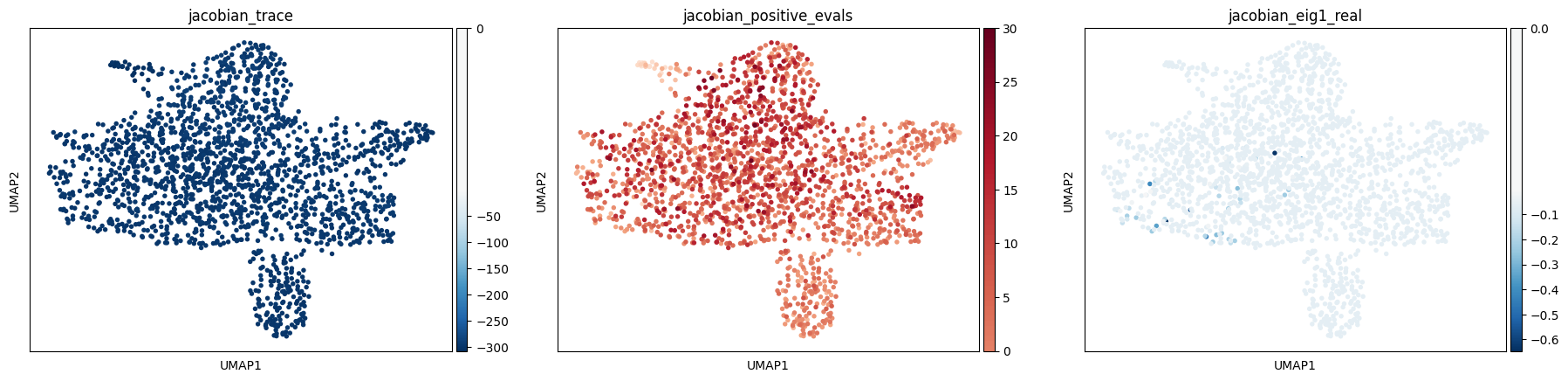
[36]:
# Visualise on UMAP
sc.pl.umap(
    adata,
    color=['jacobian_trace', 'jacobian_positive_evals', 'jacobian_eig1_real'],
    ncols=3,
    cmap='RdBu_r',
    vcenter=0
)
[37]:
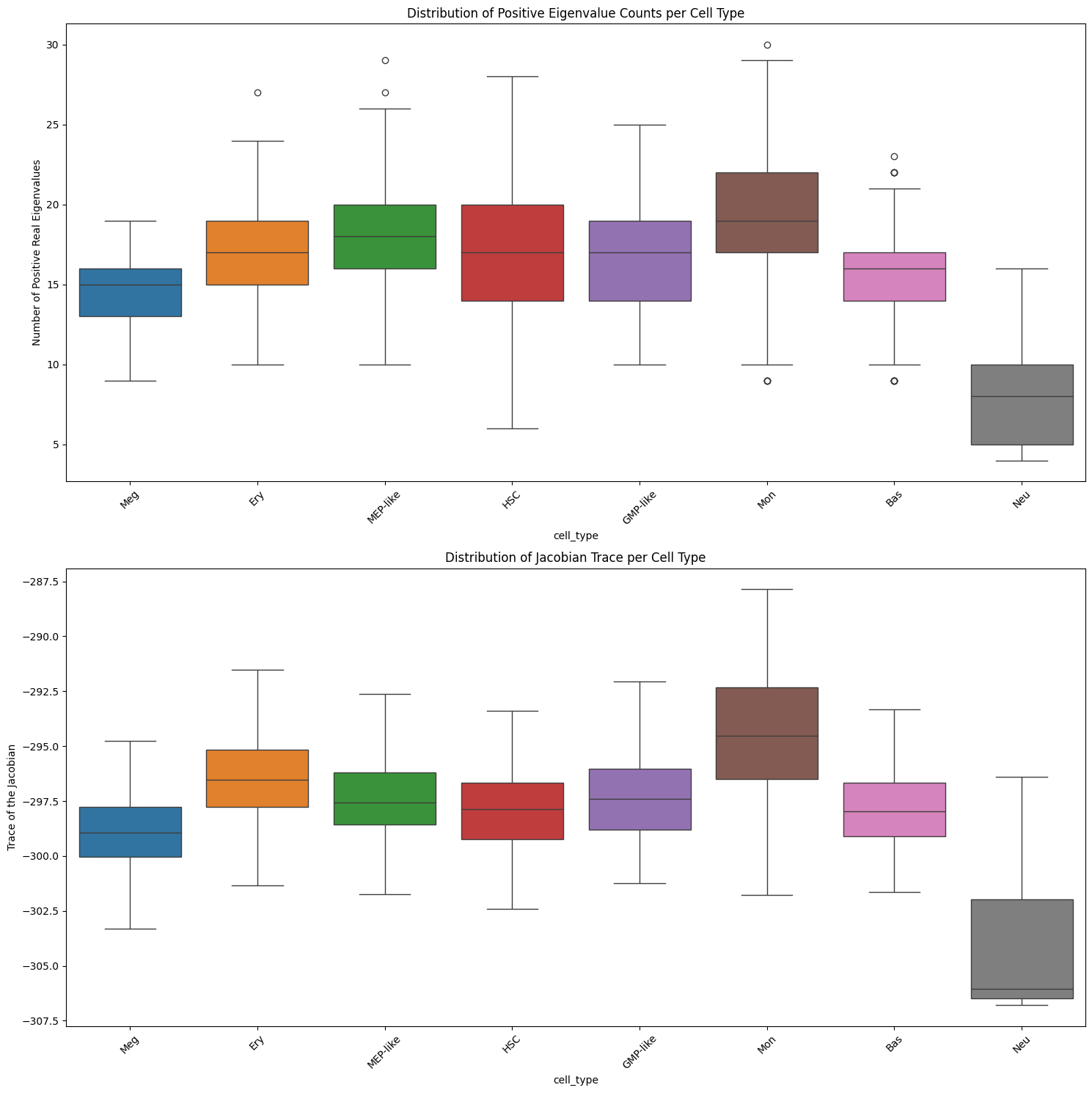
# Summary per cluster
summary = adata.obs.groupby(CLUSTER_KEY).agg({
    'jacobian_positive_evals': ['mean', 'std'],
    'jacobian_negative_evals': ['mean', 'std'],
    'jacobian_trace':          ['mean', 'std'],
})
print("\nJacobian Statistics Summary:")
summary.round(3)
Jacobian Statistics Summary:
[37]:
| jacobian_positive_evals | jacobian_negative_evals | jacobian_trace | ||||
|---|---|---|---|---|---|---|
| mean | std | mean | std | mean | std | |
| cell_type | ||||||
| Bas | 15.492 | 3.010 | 1712.508 | 3.010 | -297.896 | 1.907 |
| Ery | 17.350 | 3.096 | 1710.650 | 3.096 | -296.432 | 2.021 |
| GMP-like | 16.832 | 3.218 | 1711.168 | 3.218 | -297.408 | 1.934 |
| HSC | 17.317 | 3.969 | 1710.683 | 3.969 | -297.905 | 1.739 |
| MEP-like | 17.998 | 3.471 | 1710.002 | 3.471 | -297.345 | 1.852 |
| Meg | 14.649 | 2.138 | 1713.351 | 2.138 | -298.837 | 1.759 |
| Mon | 19.390 | 3.950 | 1708.610 | 3.950 | -294.455 | 2.827 |
| Neu | 8.219 | 3.405 | 1719.781 | 3.405 | -304.415 | 2.780 |
4.3 Eigenvalue Spectra
[38]:
# Eigenvalue spectrum in the complex plane (per cluster)
fig = sch.pl.plot_jacobian_eigenvalue_spectrum(
    adata,
    cluster_key=CLUSTER_KEY,
    order=CELL_TYPE_ORDER,
    colors=colors,
    figsize=(15, 15)
)
plt.show()

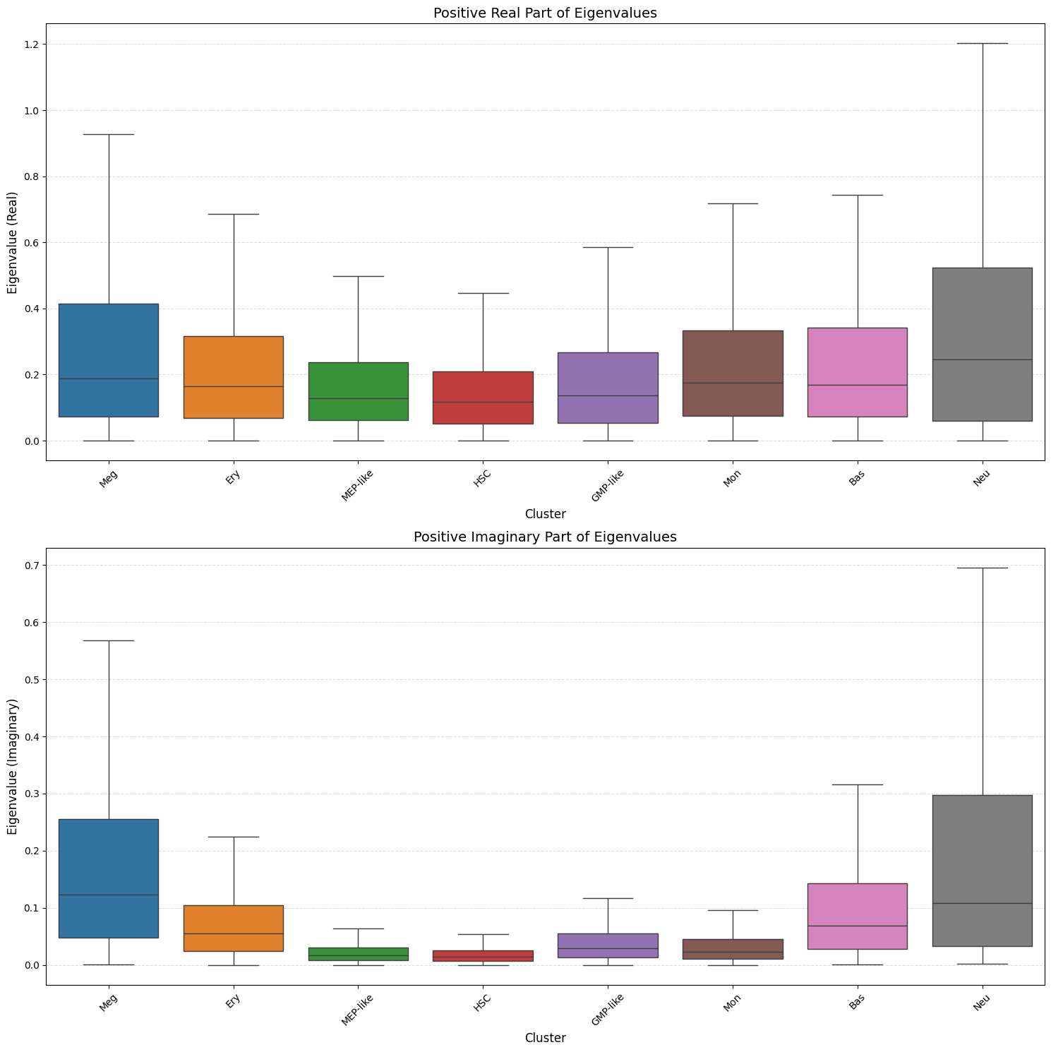
[39]:
# Boxplots of positive eigenvalue counts
fig = sch.pl.plot_jacobian_eigenvalue_boxplots(
    adata,
    cluster_key=CLUSTER_KEY,
    order=CELL_TYPE_ORDER,
    colors=colors,
    figsize=(15, 15)
)
plt.show()
[40]:
# Jacobian summary statistics as boxplots
fig = sch.pl.plot_jacobian_stats_boxplots(
    adata,
    cluster_key=CLUSTER_KEY,
    order=CELL_TYPE_ORDER,
    colors=colors,
    figsize=(15, 15)
)
plt.show()
[41]:
# Print extreme eigenvalues per cluster
print("Extreme eigenvalues per cluster:")
eigenvalues = adata.obsm['jacobian_eigenvalues']
for cluster in CELL_TYPE_ORDER:
    mask = (adata.obs[CLUSTER_KEY] == cluster).values
    evals_cluster = eigenvalues[mask]
    max_real = evals_cluster.real.max()
    min_real = evals_cluster.real.min()
    print(f"  {cluster:15s} | Max Re(λ): {max_real:8.3f} | Min Re(λ): {min_real:8.3f}")
Extreme eigenvalues per cluster:
  Meg             | Max Re(λ):    2.100 | Min Re(λ):   -1.309
  Ery             | Max Re(λ):    2.363 | Min Re(λ):   -1.257
  MEP-like        | Max Re(λ):    1.216 | Min Re(λ):   -1.257
  HSC             | Max Re(λ):    0.957 | Min Re(λ):   -1.257
  GMP-like        | Max Re(λ):    1.492 | Min Re(λ):   -1.257
  Mon             | Max Re(λ):    2.645 | Min Re(λ):   -1.257
  Bas             | Max Re(λ):    2.294 | Min Re(λ):   -1.257
  Neu             | Max Re(λ):    4.918 | Min Re(λ):   -3.191
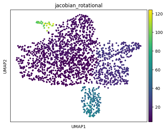
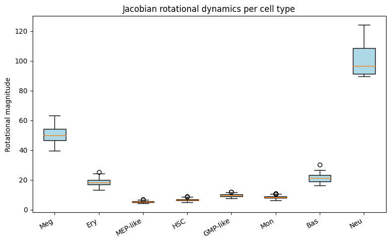
4.4 Rotational Dynamics
The antisymmetric part of J generates rotation in gene-expression phase space.
High rotational magnitude → oscillatory / spiralling dynamics near the cell state.
[42]:
sch.tl.compute_rotational_part(
    adata,
    spliced_key=SPLICED_KEY,
    cluster_key=CLUSTER_KEY,
    device=device
)

print("Rotational magnitude stored in adata.obs['jacobian_rotational']")
Computing rotational part for cluster Mon
Cluster Mon: 100%|██████████| 423/423 [00:00<00:00, 1968.56it/s]
Computing rotational part for cluster Meg
Cluster Meg: 100%|██████████| 154/154 [00:00<00:00, 4001.06it/s]
Computing rotational part for cluster MEP-like
Cluster MEP-like: 100%|██████████| 457/457 [00:00<00:00, 4010.43it/s]
Computing rotational part for cluster Ery
Cluster Ery: 100%|██████████| 234/234 [00:00<00:00, 4060.78it/s]
Computing rotational part for cluster Bas
Cluster Bas: 100%|██████████| 177/177 [00:00<00:00, 4075.27it/s]
Computing rotational part for cluster GMP-like
Cluster GMP-like: 100%|██████████| 161/161 [00:00<00:00, 4086.16it/s]
Computing rotational part for cluster HSC
Cluster HSC: 100%|██████████| 309/309 [00:00<00:00, 4231.57it/s]
Computing rotational part for cluster Neu
Cluster Neu: 100%|██████████| 32/32 [00:00<00:00, 4046.36it/s]
Rotational magnitude stored in adata.obs['jacobian_rotational']
[43]:
# Visualise rotational magnitude per cluster
sc.pl.umap(adata, color='jacobian_rotational', cmap='viridis')

# Boxplots
import matplotlib.pyplot as plt

fig, ax = plt.subplots(figsize=(8, 5), tight_layout=True)
data = [adata.obs.loc[adata.obs[CLUSTER_KEY] == ct, 'jacobian_rotational'].values
        for ct in CELL_TYPE_ORDER]
ax.boxplot(data, labels=CELL_TYPE_ORDER, patch_artist=True,
           boxprops=dict(facecolor='lightblue'))
ax.set_xticklabels(CELL_TYPE_ORDER, rotation=30, ha='right')
ax.set_ylabel('Rotational magnitude')
ax.set_title('Jacobian rotational dynamics per cell type')
plt.show()
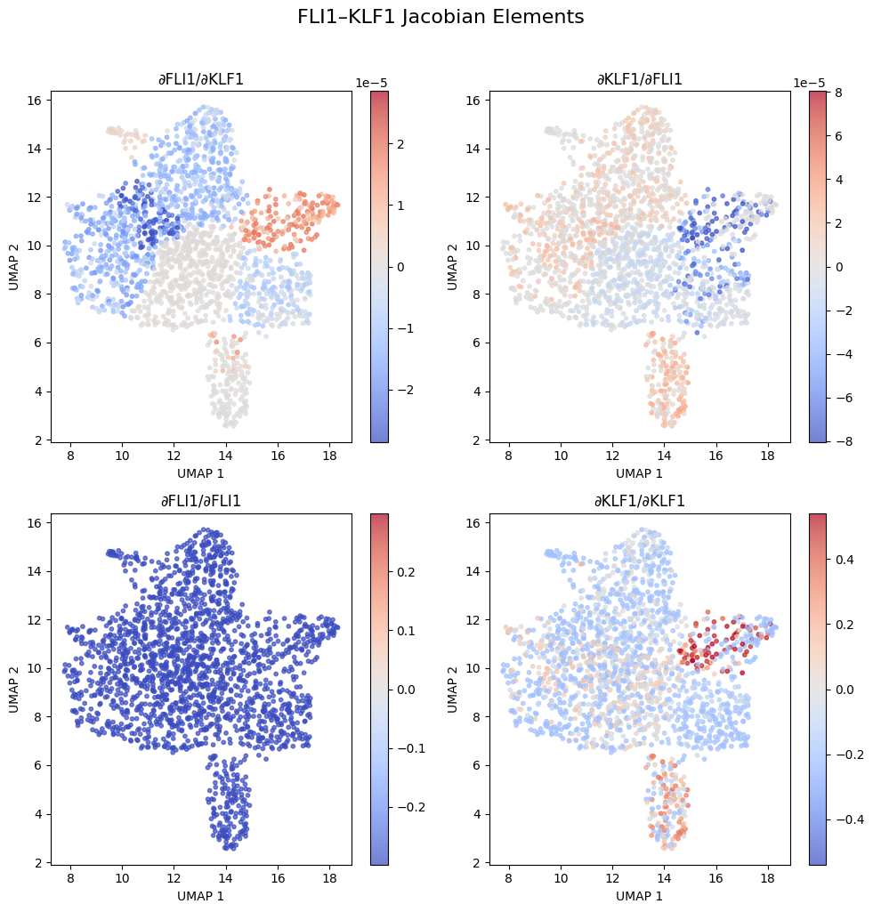
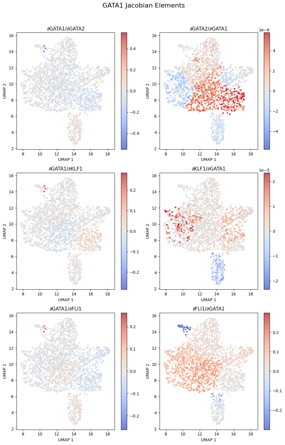
4.5 Element-wise Jacobian Analysis
Compute specific partial derivatives ∂ẋᵢ/∂xⱼ for biologically motivated
gene pairs, and visualise them on the UMAP.
[44]:
gene_pairs = [
    ('FLI1',  'KLF1'),  ('KLF1',  'FLI1'),
    ('FLI1',  'FLI1'),  ('KLF1',  'KLF1'),
    ('GATA1', 'GATA2'), ('GATA2', 'GATA1'),
    ('GATA1', 'KLF1'),  ('KLF1',  'GATA1'),
    ('GATA1', 'FLI1'),  ('FLI1',  'GATA1'),
    ('CEBPA', 'RUNX1'), ('RUNX1', 'CEBPA'),
    ('CEBPA', 'GATA2'), ('GATA2', 'CEBPA'),
    ('GATA2', 'RUNX1'), ('RUNX1', 'GATA2'),
    ('GATA2', 'GATA2'), ('RUNX1', 'RUNX1'),
]

sch.tl.compute_jacobian_elements(
    adata,
    gene_pairs=gene_pairs,
    spliced_key=SPLICED_KEY,
    cluster_key=CLUSTER_KEY,
    device=device,
    store_in_obs=True
)

print("Jacobian elements stored in adata.obs with names like: jacobian_df_GATA1_dx_GATA2")
Computing Jacobian elements for cluster Mon
Cluster Mon: 100%|██████████| 423/423 [00:01<00:00, 418.46it/s]
Computing Jacobian elements for cluster Meg
Cluster Meg: 100%|██████████| 154/154 [00:00<00:00, 479.46it/s]
Computing Jacobian elements for cluster MEP-like
Cluster MEP-like: 100%|██████████| 457/457 [00:01<00:00, 444.94it/s]
Computing Jacobian elements for cluster Ery
Cluster Ery: 100%|██████████| 234/234 [00:00<00:00, 491.22it/s]
Computing Jacobian elements for cluster Bas
Cluster Bas: 100%|██████████| 177/177 [00:00<00:00, 470.28it/s]
Computing Jacobian elements for cluster GMP-like
Cluster GMP-like: 100%|██████████| 161/161 [00:00<00:00, 442.30it/s]
Computing Jacobian elements for cluster HSC
Cluster HSC: 100%|██████████| 309/309 [00:00<00:00, 434.37it/s]
Computing Jacobian elements for cluster Neu
Cluster Neu: 100%|██████████| 32/32 [00:00<00:00, 493.67it/s]
Jacobian elements stored in adata.obs with names like: jacobian_df_GATA1_dx_GATA2
[45]:
# FLI1–KLF1 mutual regulation
fig = sch.pl.plot_jacobian_element_grid(
    adata,
    gene_pairs=[('FLI1', 'KLF1'), ('KLF1', 'FLI1'),
                ('FLI1', 'FLI1'), ('KLF1', 'KLF1')],
    ncols=2,
    figsize=(10, 10),
    s=10,
    alpha=0.7
)
plt.suptitle('FLI1–KLF1 Jacobian Elements', fontsize=16, y=1.02)
plt.show()
[46]:
# GATA1 regulon
fig = sch.pl.plot_jacobian_element_grid(
    adata,
    gene_pairs=[('GATA1', 'GATA2'), ('GATA2', 'GATA1'),
                ('GATA1', 'KLF1'),  ('KLF1',  'GATA1'),
                ('GATA1', 'FLI1'),  ('FLI1',  'GATA1')],
    ncols=2,
    figsize=(10, 15),
    s=10,
    alpha=0.7
)
plt.suptitle('GATA1 Jacobian Elements', fontsize=16, y=1.02)
plt.show()
[47]:
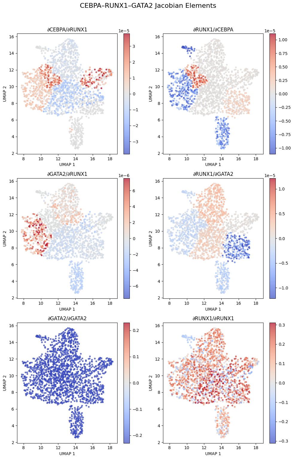
# CEBPA–RUNX1–GATA2 cross-regulation
fig = sch.pl.plot_jacobian_element_grid(
    adata,
    gene_pairs=[('CEBPA', 'RUNX1'), ('RUNX1', 'CEBPA'),
                ('GATA2', 'RUNX1'), ('RUNX1', 'GATA2'),
                ('GATA2', 'GATA2'), ('RUNX1', 'RUNX1')],
    ncols=2,
    figsize=(10, 15),
    s=10,
    alpha=0.7
)
plt.suptitle('CEBPA–RUNX1–GATA2 Jacobian Elements', fontsize=16, y=1.02)
plt.show()