This page was generated from docs/notebooks/03_network_analysis.ipynb.
Network Analysis
Network Analysis
Analyze gene regulatory network topology using centrality metrics, eigenanalysis, and network comparison.
Network Centrality
Compute centrality metrics for all genes:
This notebook analyses the structure of the inferred gene regulatory networks
(GRNs) stored in adata.varp['W_<cluster>'].
Topics covered:
Network correlation dendrograms
Symmetricity of W matrices
Network centrality (degree, betweenness, eigenvector)
Eigenanalysis of interaction matrices
GRN visualisation
Setup
[ ]:
import matplotlib.pyplot as plt
import numpy as np
import pandas as pd
import scanpy as sc
import scipy as scp
from scipy.spatial.distance import squareform
import scHopfield as sch

DATA_PATH    = './scratch/Data/'
DATASET_FILE = 'hematopoiesis.h5ad'
MODEL_FILE   = 'model.h5sch'

CLUSTER_KEY = 'cell_type'
SPLICED_KEY  = 'M_t'

CELL_TYPE_ORDER = ['Meg', 'Ery', 'MEP-like', 'HSC', 'GMP-like', 'Mon', 'Bas', 'Neu']

adata = sc.read_h5ad(DATA_PATH + DATASET_FILE)
adata = sch.tl.load_model(adata, MODEL_FILE)
print(adata)

# Cell-type colour palette
colors = dict(zip(CELL_TYPE_ORDER, adata.uns['cell_type_colors']))


# Set seed for reproducibility
np.random.seed(42)
/tmp/ipykernel_1221845/4162748082.py:19: UserWarning: adata has 1956 genes but the model was trained on 1728.  A subsetted copy is being returned; the original adata is NOT modified.  Reassign the return value:
    adata = sch.tl.load_model(adata, filename)
  adata = sch.tl.load_model(adata, MODEL_FILE)
Model loaded from 'model.h5sch'  |  clusters=['Bas', 'Ery', 'GMP-like', 'HSC', 'MEP-like', 'Meg', 'Mon', 'Neu', 'all']  |  genes=1728
AnnData object with n_obs × n_vars = 1947 × 1728
    obs: 'batch', 'time', 'cell_type', 'nGenes', 'nCounts', 'pMito', 'pass_basic_filter', 'new_Size_Factor', 'initial_new_cell_size', 'total_Size_Factor', 'initial_total_cell_size', 'spliced_Size_Factor', 'initial_spliced_cell_size', 'unspliced_Size_Factor', 'initial_unspliced_cell_size', 'Size_Factor', 'initial_cell_size', 'ntr', 'cell_cycle_phase', 'leiden', 'control_point_pca', 'inlier_prob_pca', 'obs_vf_angle_pca', 'pca_ddhodge_div', 'pca_ddhodge_potential', 'acceleration_pca', 'curvature_pca', 'n_counts', 'mt_frac', 'jacobian_det_pca', 'manual_selection', 'divergence_pca', 'curv_leiden', 'curv_louvain', 'SPI1->GATA1_jacobian', 'jacobian', 'umap_ori_leiden', 'umap_ori_louvain', 'umap_ddhodge_div', 'umap_ddhodge_potential', 'curl_umap', 'divergence_umap', 'acceleration_umap', 'control_point_umap_ori', 'inlier_prob_umap_ori', 'obs_vf_angle_umap_ori', 'curvature_umap_ori'
    var: 'gene_name', 'gene_id', 'nCells', 'nCounts', 'pass_basic_filter', 'use_for_pca', 'frac', 'ntr', 'time_3_alpha', 'time_3_beta', 'time_3_gamma', 'time_3_half_life', 'time_3_alpha_b', 'time_3_alpha_r2', 'time_3_gamma_b', 'time_3_gamma_r2', 'time_3_gamma_logLL', 'time_3_delta_b', 'time_3_delta_r2', 'time_3_bs', 'time_3_bf', 'time_3_uu0', 'time_3_ul0', 'time_3_su0', 'time_3_sl0', 'time_3_U0', 'time_3_S0', 'time_3_total0', 'time_3_beta_k', 'time_3_gamma_k', 'time_5_alpha', 'time_5_beta', 'time_5_gamma', 'time_5_half_life', 'time_5_alpha_b', 'time_5_alpha_r2', 'time_5_gamma_b', 'time_5_gamma_r2', 'time_5_gamma_logLL', 'time_5_bs', 'time_5_bf', 'time_5_uu0', 'time_5_ul0', 'time_5_su0', 'time_5_sl0', 'time_5_U0', 'time_5_S0', 'time_5_total0', 'time_5_beta_k', 'time_5_gamma_k', 'use_for_dynamics', 'gamma', 'gamma_r2', 'use_for_transition', 'gamma_k', 'gamma_b', 'I_Bas', 'I_Ery', 'I_GMP-like', 'I_HSC', 'I_MEP-like', 'I_Meg', 'I_Mon', 'I_Neu', 'I_all', 'scHopfield_used', 'sigmoid_exponent', 'sigmoid_mse', 'sigmoid_offset', 'sigmoid_threshold'
    uns: 'PCs', 'VecFld_pca', 'VecFld_umap', 'X_umap_neighbors', 'cell_phase_genes', 'cell_type_colors', 'dynamics', 'explained_variance_ratio_', 'feature_selection', 'grid_velocity_pca', 'grid_velocity_umap', 'grid_velocity_umap_ori_perturbation', 'grid_velocity_umap_test', 'jacobian_pca', 'leiden', 'neighbors', 'pca_mean', 'pp', 'response', 'scHopfield'
    obsm: 'X', 'X_pca', 'X_pca_SparseVFC', 'X_umap', 'X_umap_SparseVFC', 'X_umap_ori_perturbation', 'X_umap_test', 'acceleration_pca', 'acceleration_umap', 'cell_cycle_scores', 'curvature_pca', 'curvature_umap', 'j_delta_x_perturbation', 'velocity_pca', 'velocity_pca_SparseVFC', 'velocity_umap', 'velocity_umap_SparseVFC', 'velocity_umap_ori_perturbation', 'velocity_umap_test'
    layers: 'M_n', 'M_nn', 'M_t', 'M_tn', 'M_tt', 'X_new', 'X_total', 'velocity_alpha_minus_gamma_s'
    obsp: 'X_umap_connectivities', 'X_umap_distances', 'connectivities', 'cosine_transition_matrix', 'distances', 'fp_transition_rate', 'moments_con', 'pca_ddhodge', 'perturbation_transition_matrix', 'umap_ddhodge'
    varp: 'W_Bas', 'W_Ery', 'W_GMP-like', 'W_HSC', 'W_MEP-like', 'W_Meg', 'W_Mon', 'W_Neu', 'W_all'
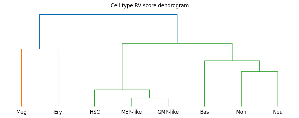
3.1 Network Correlation Dendrograms
Compute pairwise similarity between cell-type networks using the RV coefficient
and Pearson / Hamming distances.
[16]:
# Cell-type similarity based on expression covariance (RV score)
sch.tl.celltype_correlation(
    adata,
    spliced_key=SPLICED_KEY,
    cluster_key=CLUSTER_KEY
)

cells_correlation = adata.uns['scHopfield']['celltype_correlation']

fig, ax = plt.subplots(figsize=(10, 4), tight_layout=True)
Z = scp.cluster.hierarchy.linkage(squareform(1 - cells_correlation), 'complete')
scp.cluster.hierarchy.dendrogram(Z, labels=cells_correlation.index, ax=ax)
for spine in ax.spines.values():
    spine.set_visible(False)
ax.get_yaxis().set_visible(False)
ax.set_title('Cell-type RV score dendrogram')
plt.show()
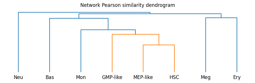
[17]:
# Network-structure similarity (W matrix correlations)
sch.tl.network_correlations(adata, cluster_key=CLUSTER_KEY)

pearson    = adata.uns['scHopfield']['network_correlations']['pearson']
hamming    = adata.uns['scHopfield']['network_correlations']['hamming']
pearson_bin = adata.uns['scHopfield']['network_correlations']['pearson_bin']

fig, ax = plt.subplots(figsize=(9, 3), tight_layout=True)
for spine in ax.spines.values():
    spine.set_visible(False)
ax.get_yaxis().set_visible(False)

Z = scp.cluster.hierarchy.linkage(squareform(1 - pearson), 'complete')
scp.cluster.hierarchy.dendrogram(Z, labels=pearson.index, ax=ax)
ax.set_title('Network Pearson similarity dendrogram')
plt.show()
/home/bernaljp/miniconda3/envs/SCH/lib/python3.11/site-packages/numpy/lib/function_base.py:2897: RuntimeWarning: invalid value encountered in divide
  c /= stddev[:, None]
/home/bernaljp/miniconda3/envs/SCH/lib/python3.11/site-packages/numpy/lib/function_base.py:2898: RuntimeWarning: invalid value encountered in divide
  c /= stddev[None, :]
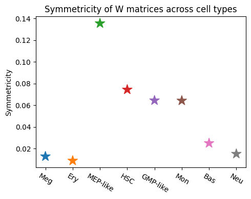
3.2 Symmetricity Analysis
A symmetric W ≈ equilibrium system; a skew-symmetric W ≈ oscillatory system.
The symmetricity score ranges from −1 (fully skew-symmetric) to +1 (fully
symmetric).
[18]:
def symmetricity(A, norm=2):
    """Ratio of symmetric to total Frobenius norm."""
    S  = np.linalg.norm((A + A.T) / 2, ord=norm)
    As = np.linalg.norm((A - A.T) / 2, ord=norm)
    return (S - As) / (S + As)

genes_used = adata.var['use_for_dynamics'].values
W = {
    cluster: adata.varp[f'W_{cluster}'][genes_used][:, genes_used]
    for cluster in CELL_TYPE_ORDER
}

syms = np.array([symmetricity(W[k]) for k in CELL_TYPE_ORDER])

fig, ax = plt.subplots(figsize=(5, 4), tight_layout=True)
ax.scatter(
    range(len(CELL_TYPE_ORDER)), syms, s=200, marker='*',
    c=[colors[k] for k in CELL_TYPE_ORDER]
)
ax.set_xticks(range(len(CELL_TYPE_ORDER)))
ax.set_xticklabels(CELL_TYPE_ORDER, rotation=-30)
ax.set_ylabel('Symmetricity')
ax.set_title('Symmetricity of W matrices across cell types')
plt.show()
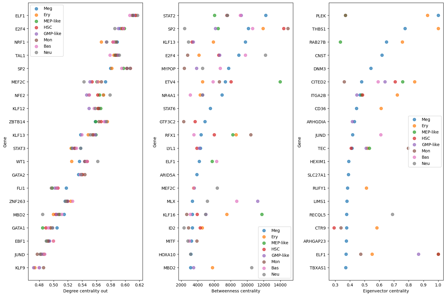
3.3 Network Centrality
Three complementary centrality measures:
degree_centrality_out: fraction of outgoing edges
betweenness_centrality: fraction of shortest paths through node
eigenvector_centrality: influence weighted by neighbour importance
[19]:
sch.tl.compute_network_centrality(
    adata,
    cluster_key=CLUSTER_KEY,
    threshold_number=40000   # keep top-N edges per cluster
)
/home/bernaljp/packages/scHopfield/scHopfield/tools/networks.py:304: RuntimeWarning: Some eigenvector centralities are nearly zero, indicating that the graph may not be (strongly) connected. Eigenvector centrality is not meaningful for disconnected graphs. Location: src/centrality/eigenvector.c:102
  result_df["eigenvector_centrality"] = g.eigenvector_centrality(directed=True, weights="weight")
[20]:
# Ranked gene plots for each metric
fig, axes = plt.subplots(1, 3, figsize=(15, 10))

metrics = ['degree_centrality_out', 'betweenness_centrality', 'eigenvector_centrality']
for ax, metric in zip(axes, metrics):
    sch.pl.plot_network_centrality_rank(
        adata,
        metric=metric,
        clusters=CELL_TYPE_ORDER,
        cluster_key=CLUSTER_KEY,
        n_genes=20,
        colors=colors,
        ax=ax
    )
plt.tight_layout()
plt.show()
[23]:
# Top-gene tables
df_betweenness = sch.tl.get_top_genes_table(
    adata,
    metric='betweenness_centrality',
    cluster_key=CLUSTER_KEY,
    n_genes=20,
    order=CELL_TYPE_ORDER
)
print("Betweenness centrality top genes:")
df_betweenness
Betweenness centrality top genes:
[23]:
| Meg | Ery | MEP-like | HSC | GMP-like | Mon | Bas | Neu | |||||||||
|---|---|---|---|---|---|---|---|---|---|---|---|---|---|---|---|---|
| Gene | Betweenness Centrality | Gene | Betweenness Centrality | Gene | Betweenness Centrality | Gene | Betweenness Centrality | Gene | Betweenness Centrality | Gene | Betweenness Centrality | Gene | Betweenness Centrality | Gene | Betweenness Centrality | |
| 0 | STAT2 | 12250.0 | SP2 | 11927.0 | ETV4 | 13980.5 | KLF9 | 14669.0 | MLX | 11277.0 | SP2 | 14913.0 | SP2 | 10643.0 | NRF1 | 13401.0 |
| 1 | SP2 | 10144.0 | RFX1 | 8652.0 | KLF16 | 11760.5 | SP2 | 14413.0 | STAT2 | 9261.0 | RFX1 | 10432.0 | E2F4 | 9778.0 | E2F4 | 12196.0 |
| 2 | KLF13 | 9788.0 | KLF16 | 7518.0 | NRF1 | 11469.0 | ETV4 | 8021.0 | KLF9 | 7476.0 | TCF3 | 9838.0 | STAT2 | 9155.0 | JUND | 11289.0 |
| 3 | E2F4 | 8986.0 | KLF9 | 7180.0 | CUX1 | 8931.5 | AHRR | 7765.0 | E2F4 | 6669.0 | STAT2 | 7591.0 | MLX | 8709.0 | MBD2 | 10526.0 |
| 4 | MYPOP | 7762.0 | JUND | 6566.0 | RFX1 | 8260.0 | STAT2 | 7544.0 | SP2 | 6167.0 | NRF1 | 7298.0 | ATF6B | 7185.0 | TCF3 | 8086.0 |
| 5 | ETV4 | 7360.0 | STAT3 | 6291.0 | ATF6B | 6912.0 | EBF1 | 6844.0 | ZBTB4 | 5963.0 | ETV4 | 6633.0 | HIVEP1 | 7116.0 | STAT2 | 7568.0 |
| 6 | NR4A1 | 6963.0 | NRF1 | 6190.0 | SP2 | 6479.0 | E2F4 | 6531.0 | NFE2 | 5612.0 | MYCN | 5684.0 | MYPOP | 6732.0 | MEF2C | 6378.0 |
| 7 | STAT6 | 5544.0 | KLF13 | 5881.0 | STAT2 | 6031.0 | NRF1 | 6247.0 | KLF16 | 4984.0 | KLF9 | 5648.0 | ELF1 | 6284.0 | MLX | 5159.0 |
| 8 | GTF3C2 | 4864.0 | HIVEP1 | 5876.0 | ELF1 | 5746.0 | RFX1 | 5999.0 | EBF1 | 4781.0 | AHRR | 4976.0 | AHRR | 5959.0 | KLF16 | 4968.0 |
| 9 | RFX1 | 4404.0 | MBD2 | 5777.0 | EBF1 | 5078.5 | JUND | 5013.0 | NR4A1 | 4596.0 | STAT3 | 4830.0 | ETV4 | 5845.0 | ETV6 | 4868.0 |
| 10 | LYL1 | 4319.0 | WT1 | 4853.0 | HLF | 4986.0 | STAT3 | 4977.0 | KLF1 | 4582.0 | ZBTB4 | 4139.0 | TCF3 | 5841.0 | MYPOP | 4574.0 |
| 11 | ELF1 | 4196.0 | ETV4 | 4590.0 | NR4A1 | 4575.0 | ID2 | 4289.0 | ITGB2 | 4474.0 | MITF | 3906.0 | NRF1 | 3816.0 | STAT3 | 4389.0 |
| 12 | ARID5A | 3900.0 | ID2 | 4564.0 | AHRR | 4477.0 | MEIS1 | 3983.0 | LYL1 | 4175.0 | NFE2 | 3305.0 | POU6F1 | 3564.0 | ZBTB4 | 3418.0 |
| 13 | MEF2C | 3583.0 | NFE2 | 4552.0 | POU6F1 | 4411.0 | KLF16 | 3947.0 | NRF1 | 3993.0 | CEBPA | 2909.0 | MEF2C | 3553.0 | MEF2D | 3299.0 |
| 14 | MLX | 3372.0 | NR4A1 | 4284.0 | JUND | 4033.5 | LYL1 | 3914.0 | MYPOP | 3870.0 | ID2 | 2891.0 | RFX1 | 3552.0 | HOXA10 | 3142.0 |
| 15 | KLF16 | 3349.0 | ETV6 | 4188.0 | ZBTB4 | 3943.0 | TCF3 | 3798.0 | AHRR | 3767.0 | E2F4 | 2764.0 | GATA1 | 3436.0 | KLF13 | 2876.0 |
| 16 | ID2 | 3348.0 | E2F4 | 4160.0 | TCF3 | 3794.0 | WT1 | 3706.0 | MBD2 | 3487.0 | KLF16 | 2654.0 | NFE2 | 3120.0 | MITF | 2797.0 |
| 17 | MITF | 3261.0 | TCF3 | 3910.0 | FOSL2 | 3654.0 | GTF3C2 | 3684.0 | KLF13 | 3468.0 | MYPOP | 2362.0 | NR4A1 | 3105.0 | FLI1 | 2709.0 |
| 18 | HOXA10 | 3191.0 | CUX1 | 3501.0 | KLF9 | 3516.0 | HIVEP1 | 3572.0 | CUX1 | 3447.0 | GTF3C2 | 2322.0 | KLF16 | 3098.0 | SP2 | 2428.0 |
| 19 | MBD2 | 3124.0 | MEF2C | 3495.0 | STAT3 | 3244.0 | KLF13 | 3336.0 | HIVEP1 | 3442.0 | MEF2D | 2297.0 | MITF | 2985.0 | ID2 | 2335.0 |
[24]:
df_degree = sch.tl.get_top_genes_table(
    adata,
    metric='degree_centrality_out',
    cluster_key=CLUSTER_KEY,
    n_genes=20,
    order=CELL_TYPE_ORDER
)
print("\nDegree centrality top genes:")
df_degree
Degree centrality top genes:
[24]:
| Meg | Ery | MEP-like | HSC | GMP-like | Mon | Bas | Neu | |||||||||
|---|---|---|---|---|---|---|---|---|---|---|---|---|---|---|---|---|
| Gene | Degree Centrality Out | Gene | Degree Centrality Out | Gene | Degree Centrality Out | Gene | Degree Centrality Out | Gene | Degree Centrality Out | Gene | Degree Centrality Out | Gene | Degree Centrality Out | Gene | Degree Centrality Out | |
| 0 | ELF1 | 0.612044 | ELF1 | 0.614360 | ELF1 | 0.610886 | ELF1 | 0.614939 | ELF1 | 0.612044 | ELF1 | 0.609728 | ELF1 | 0.606254 | ELF1 | 0.617255 |
| 1 | E2F4 | 0.592936 | E2F4 | 0.595252 | E2F4 | 0.598726 | SP2 | 0.607412 | SP2 | 0.602779 | SP2 | 0.602200 | E2F4 | 0.597568 | SP2 | 0.606833 |
| 2 | NRF1 | 0.588882 | TAL1 | 0.584250 | SP2 | 0.597568 | E2F4 | 0.597568 | E2F4 | 0.590620 | E2F4 | 0.595831 | SP2 | 0.595252 | TAL1 | 0.591778 |
| 3 | TAL1 | 0.586566 | SP2 | 0.581355 | TAL1 | 0.587145 | TAL1 | 0.588882 | TAL1 | 0.590041 | NRF1 | 0.587724 | NRF1 | 0.583671 | E2F4 | 0.585408 |
| 4 | SP2 | 0.579618 | ZBTB14 | 0.574986 | NRF1 | 0.585408 | NRF1 | 0.583092 | NRF1 | 0.573827 | TAL1 | 0.585987 | TAL1 | 0.579039 | NFE2 | 0.579039 |
| 5 | MEF2C | 0.572669 | NFE2 | 0.569774 | KLF12 | 0.565721 | ZBTB14 | 0.566300 | ZBTB14 | 0.572090 | MEF2C | 0.566879 | ZBTB14 | 0.570932 | NRF1 | 0.574406 |
| 6 | NFE2 | 0.569774 | NRF1 | 0.566879 | NFE2 | 0.563984 | KLF12 | 0.562247 | KLF13 | 0.558193 | ZBTB14 | 0.563405 | MEF2C | 0.561089 | ZBTB14 | 0.573827 |
| 7 | KLF12 | 0.563405 | MEF2C | 0.562247 | MEF2C | 0.560510 | NFE2 | 0.561668 | MEF2C | 0.550666 | KLF12 | 0.563405 | KLF12 | 0.556456 | WT1 | 0.561668 |
| 8 | ZBTB14 | 0.558193 | KLF12 | 0.562247 | KLF13 | 0.559351 | KLF13 | 0.555877 | KLF12 | 0.549508 | KLF13 | 0.554140 | NFE2 | 0.550087 | KLF12 | 0.558193 |
| 9 | KLF13 | 0.537927 | KLF13 | 0.548350 | ZBTB14 | 0.558772 | MEF2C | 0.553561 | NFE2 | 0.546034 | NFE2 | 0.549508 | WT1 | 0.546613 | KLF13 | 0.551245 |
| 10 | STAT3 | 0.537927 | GATA2 | 0.539085 | WT1 | 0.546034 | WT1 | 0.547192 | WT1 | 0.543138 | GATA2 | 0.543717 | KLF13 | 0.539664 | MEF2C | 0.542559 |
| 11 | WT1 | 0.536190 | WT1 | 0.525188 | GATA2 | 0.538506 | GATA2 | 0.540243 | GATA2 | 0.537927 | WT1 | 0.543717 | GATA2 | 0.537348 | GATA2 | 0.538506 |
| 12 | GATA2 | 0.535032 | STAT3 | 0.524609 | STAT3 | 0.525767 | STAT3 | 0.529241 | STAT3 | 0.526346 | STAT3 | 0.529820 | STAT3 | 0.532137 | STAT3 | 0.537927 |
| 13 | FLI1 | 0.517661 | ZNF263 | 0.524030 | ZNF263 | 0.518819 | ZNF263 | 0.519977 | ZNF263 | 0.519398 | ZNF263 | 0.518240 | ZNF263 | 0.526346 | ZNF263 | 0.516503 |
| 14 | ZNF263 | 0.515924 | MBD2 | 0.499710 | MBD2 | 0.508396 | FLI1 | 0.506080 | MBD2 | 0.504343 | MBD2 | 0.506659 | MBD2 | 0.511291 | GATA1 | 0.498552 |
| 15 | MBD2 | 0.514765 | EBF1 | 0.499710 | FLI1 | 0.497973 | MBD2 | 0.503185 | FLI1 | 0.502027 | FLI1 | 0.504343 | FLI1 | 0.504922 | FLI1 | 0.496815 |
| 16 | GATA1 | 0.504922 | FLI1 | 0.497394 | EBF1 | 0.490446 | EBF1 | 0.492183 | GATA1 | 0.498552 | GATA1 | 0.495657 | EBF1 | 0.499710 | EBF1 | 0.489867 |
| 17 | EBF1 | 0.493341 | GATA1 | 0.496236 | GATA1 | 0.484655 | GATA1 | 0.489288 | EBF1 | 0.494499 | EBF1 | 0.492183 | GATA1 | 0.492762 | MBD2 | 0.484655 |
| 18 | JUND | 0.486972 | JUND | 0.486393 | JUND | 0.482339 | JUND | 0.482339 | JUND | 0.484076 | KLF9 | 0.485814 | JUND | 0.487551 | STAT2 | 0.484655 |
| 19 | KLF9 | 0.480023 | KLF9 | 0.473654 | STAT2 | 0.474812 | STAT2 | 0.470759 | KLF9 | 0.471917 | JUND | 0.477128 | KLF9 | 0.479444 | JUND | 0.481181 |
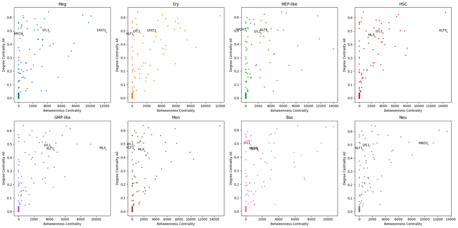
[25]:
# Betweenness vs degree scatter (high betweenness, low degree = bottleneck genes)
fig = sch.pl.plot_centrality_scatter(
    adata,
    x_metric='betweenness_centrality',
    y_metric='degree_centrality_all',
    cluster_key=CLUSTER_KEY,
    order=CELL_TYPE_ORDER,
    colors=colors,
    n_top_genes=3,
    filter_threshold=('degree_centrality_all', '<', 0.5),
    figsize=(20, 10)
)
plt.show()
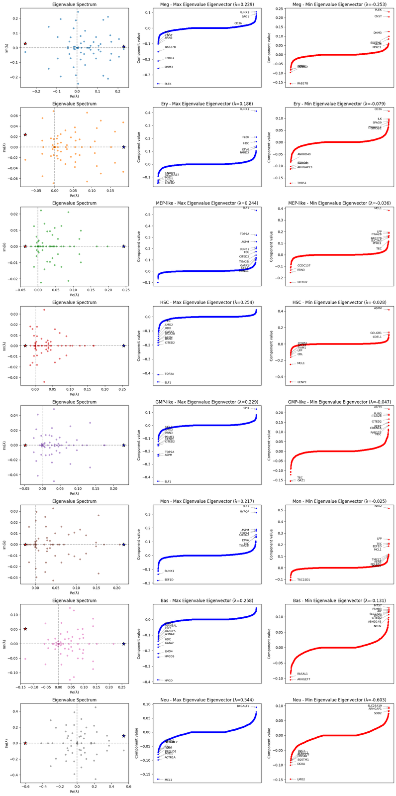
3.4 Eigenanalysis
Eigendecomposition of each cluster’s W matrix reveals:
Dominant regulatory directions (top eigenvector genes)
Stability indicators (sign of leading eigenvalue)
[26]:
sch.tl.compute_eigenanalysis(adata, cluster_key=CLUSTER_KEY)
[27]:
# Comprehensive grid: spectrum + max/min eigenvector gene loadings
fig = sch.pl.plot_eigenanalysis_grid(
    adata,
    cluster_key=CLUSTER_KEY,
    order=CELL_TYPE_ORDER,
    colors=colors,
    n_genes=10,
    figsize=(16, 4 * len(CELL_TYPE_ORDER))
)
plt.show()
[32]:
# Table of top genes from extreme eigenvectors
df_eigenanalysis = sch.tl.get_eigenanalysis_table(
    adata,
    cluster_key=CLUSTER_KEY,
    n_genes=20,
    order=CELL_TYPE_ORDER
)
df_eigenanalysis.head(10)
[32]:
| Meg | Ery | MEP-like | ... | Mon | Bas | Neu | |||||||||||||||
|---|---|---|---|---|---|---|---|---|---|---|---|---|---|---|---|---|---|---|---|---|---|
| +EV gene | +EV value | -EV gene | -EV value | +EV gene | +EV value | -EV gene | -EV value | +EV gene | +EV value | ... | -EV gene | -EV value | +EV gene | +EV value | -EV gene | -EV value | +EV gene | +EV value | -EV gene | -EV value | |
| 0 | PLEK | -0.357 | PLEK | 0.233 | RUNX1 | 0.412 | THBS1 | -0.172 | ELF1 | 0.537 | ... | NAV2 | 0.514 | HPGD | -0.387 | INTS7 | 0.130 | MCL1 | -0.168 | LMO2 | -0.148 |
| 1 | DNM3 | -0.258 | CNST | 0.205 | PLEK | 0.210 | CD36 | 0.130 | TOP2A | 0.320 | ... | LPP | 0.246 | HPGDS | -0.242 | PSMB3 | 0.123 | ACTR1A | -0.099 | DGKA | -0.101 |
| 2 | THBS1 | -0.211 | RAB27B | -0.158 | HDC | 0.175 | ARHGAP23 | -0.113 | ASPM | 0.262 | ... | TEC | 0.212 | LMO4 | -0.219 | AIP | 0.122 | MXD1 | -0.090 | SLC25A19 | 0.096 |
| 3 | RAB27B | -0.151 | DNM3 | 0.126 | CITED2 | -0.147 | RAB27B | -0.111 | CCNB1 | 0.212 | ... | EEF1D | 0.206 | GATA2 | -0.177 | SLC27A1 | 0.117 | B4GALT1 | 0.089 | SQSTM1 | -0.092 |
| 4 | RUNX1 | 0.105 | SQSTM1 | 0.099 | TCTN2 | -0.143 | ITGA2B | -0.102 | TEC | 0.200 | ... | MCL1 | 0.190 | HDC | -0.162 | SRGN | 0.117 | PRELID1 | -0.089 | ARHGAP1 | 0.092 |
| 5 | RRN3 | -0.103 | CCNB1 | -0.096 | ETV6 | 0.140 | ILK | 0.097 | CITED2 | 0.174 | ... | TMCC1 | 0.117 | AHNAK | -0.138 | CITED2 | 0.115 | TNS3 | -0.079 | UBE4A | -0.086 |
| 6 | CNST | -0.096 | TMEM229B | 0.086 | MXD1 | -0.132 | CITED2 | 0.092 | ITGA2B | 0.143 | ... | RERE | 0.113 | RASSF5 | -0.129 | ABHD14B | 0.107 | ZFPM2 | -0.073 | RHBDD3 | -0.085 |
| 7 | BAG1 | 0.091 | CD36 | 0.085 | PARD3 | 0.130 | SPAG9 | 0.088 | GATA2 | 0.121 | ... | TSC22D1 | -0.109 | ELF1 | -0.121 | ARHGEF7 | -0.105 | SNCA | 0.073 | SPECC1 | -0.085 |
| 8 | TEC | -0.089 | LDB1 | -0.083 | SLC25A37 | -0.124 | SLC25A37 | -0.083 | MCL1 | 0.113 | ... | POLR1C | 0.104 | MANBAL | -0.114 | NCLN | 0.098 | ST3GAL2 | -0.072 | TNS3 | -0.084 |
| 9 | ABHD14A | -0.087 | THBS1 | -0.081 | CNRIP1 | -0.124 | ZDHHC12 | 0.083 | RUNX1 | 0.102 | ... | PGBD5 | 0.102 | PLIN2 | -0.109 | RASAL1 | -0.096 | CPNE9 | 0.072 | SOD2 | 0.084 |
10 rows × 32 columns
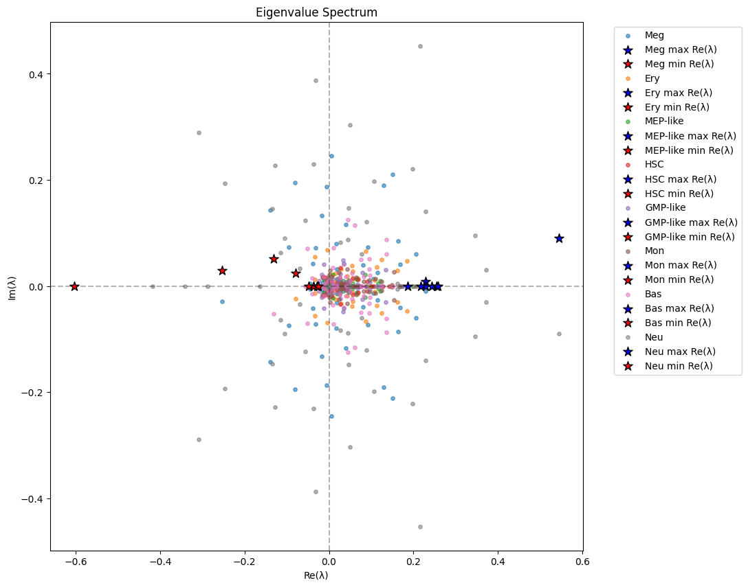
[29]:
# Eigenvalue spectra for all clusters overlaid
fig, ax = plt.subplots(figsize=(10, 10))
sch.pl.plot_eigenvalue_spectrum(
    adata,
    clusters=CELL_TYPE_ORDER,
    cluster_key=CLUSTER_KEY,
    colors=colors,
    highlight_extremes=True,
    ax=ax
)
plt.show()
[30]:
# Leading eigenvector per cluster — extreme eigenvalues summary
print("Extreme eigenvalues per cluster:")
for cluster in CELL_TYPE_ORDER:
    evals = adata.uns['scHopfield']['eigenanalysis'][f'eigenvalues_{cluster}']
    max_ev = evals[np.argmax(evals.real)]
    min_ev = evals[np.argmin(evals.real)]
    print(f"  {cluster:15s} | Max Re(λ): {max_ev.real:8.3f} | Min Re(λ): {min_ev.real:8.3f}")
Extreme eigenvalues per cluster:
  Meg             | Max Re(λ):    0.229 | Min Re(λ):   -0.253
  Ery             | Max Re(λ):    0.186 | Min Re(λ):   -0.079
  MEP-like        | Max Re(λ):    0.244 | Min Re(λ):   -0.036
  HSC             | Max Re(λ):    0.254 | Min Re(λ):   -0.028
  GMP-like        | Max Re(λ):    0.229 | Min Re(λ):   -0.047
  Mon             | Max Re(λ):    0.217 | Min Re(λ):   -0.025
  Bas             | Max Re(λ):    0.258 | Min Re(λ):   -0.131
  Neu             | Max Re(λ):    0.544 | Min Re(λ):   -0.603
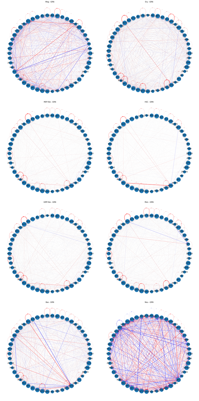
3.5 GRN Visualisation
[31]:
from matplotlib.colors import LinearSegmentedColormap

colors_graph = ['blue', 'lightgray', 'red']
custom_cmap  = LinearSegmentedColormap.from_list('custom_cmap', list(zip([0, 0.5, 1], colors_graph)))

score = 'degree_centrality_out'
topn  = 50

fig, axs = plt.subplots(4, 2, figsize=(20, 40), tight_layout=True)

for cluster, ax in zip(CELL_TYPE_ORDER, axs.flat):
    ax.axis('off')
    ax.set_title(f'{score.replace("_", " ").capitalize()} — {cluster}')
    sch.pl.plot_grn_network(
        adata,
        cluster=cluster,
        topn=topn,
        score_size=score,
        ax=ax,
        cmap=custom_cmap
    )

plt.show()